
Function map and cheat sheet
Source:vignettes/articles/function-map-cheatsheet.Rmd
function-map-cheatsheet.RmdUse this guide when you have several responses for each site,
individual, species, or study and know what you need to do next, but not
which gllvmTMB function starts that task. It is a
navigation aid, not a claim that every documented formula, family,
covariance source, or interval is suitable for every data set.
This task-based lookup guide sits within Get started because it routes readers to the current API and existing worked guides. Get started and Individual morphometrics remain the better first read when you are new to GLLVMs.
Find the next step
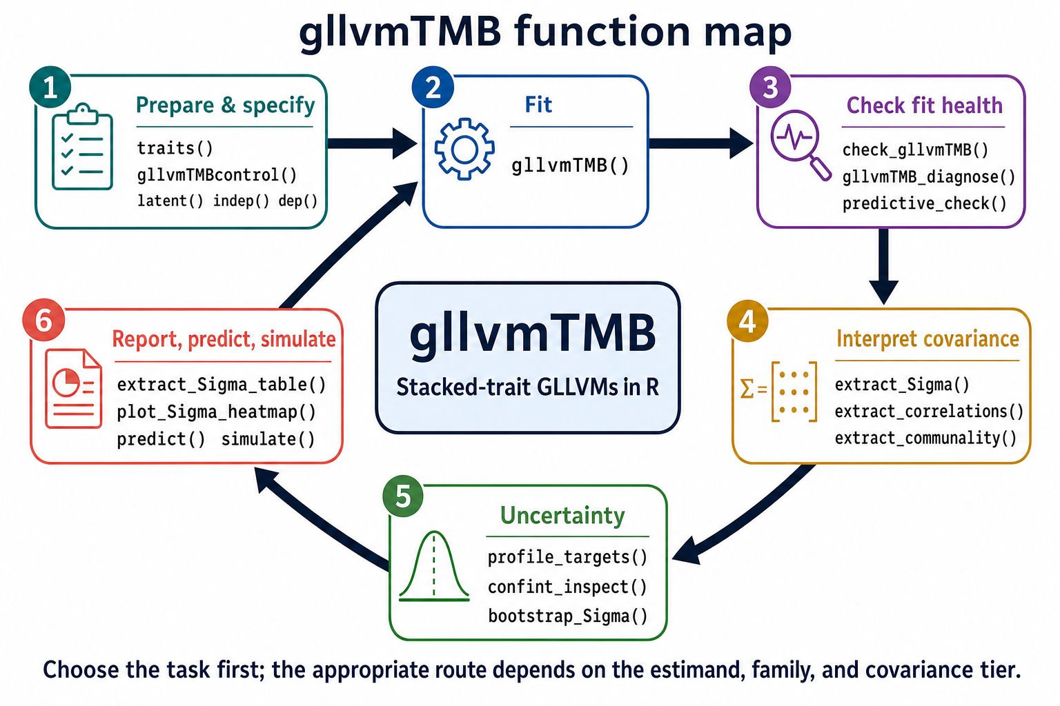
gllvmTMB function map
Choose the task first; then follow the relevant function and guide.
Step 1: Prepare and specify
Put responses into long or wide data and state the covariance question.
Prepare a modelStart with ordinary covariance; add a relationship source only when the study design supplies one.Step 2: Fit
Fit every stacked-trait model through one entry point.
Fit with gllvmTMB()Use a supported response family and retain the formula that defines the estimand.Step 3: Check fit health
Check convergence, gradients, Hessian information, and fitted-response mismatch before interpretation.
Check the fitA syntactically valid model can still be weakly identified for its data.Step 4: Interpret covariance
Extract rotation-invariant covariance, correlation, and shared-variance summaries first.
Extract a scientific quantityLoadings and ordination scores are orientation-dependent; interpret them after covariance summaries.Step 5: Choose a target-specific uncertainty route
Inspect available methods and their returned status rather than assuming a generic confidence interval.
Inspect interval supportInterval availability and calibration depend on the estimand, family, and covariance tier.Step 6: Report, predict, or simulate
Make report-ready tables and figures, predict fitted responses, or simulate new responses.
Report or predictName the target and scale in every reported table or figure.Typical route: Prepare and specify → Fit → Check fit health → Interpret covariance. Prediction, simulation, and uncertainty are conditional branches, not compulsory stages.
The cards use colour and order as helpful cues; their headings and links provide the complete reading order without colour, arrows, or CSS.
A five-minute route through the map
The smallest ordinary workflow asks whether three continuous traits
covary across sites. Here, latent() represents a low-rank
shared covariance and its ordinary default includes the trait-specific
diagonal Psi. Thus Sigma = Lambda Lambda^T + Psi;
Sigma is the model-implied trait covariance,
Lambda is the shared loading matrix, and Psi
is the diagonal of trait-specific variance.
sim <- simulate_site_trait(
  n_sites = 24, n_species = 1, n_traits = 3,
  mean_species_per_site = 1,
  Lambda_B = matrix(c(0.8, 0.5, -0.4), nrow = 3, ncol = 1),
  psi_B = c(0.3, 0.25, 0.2), seed = 20260722
)

fit <- gllvmTMB(
  value ~ 0 + trait + latent(0 + trait | site, d = 1),
  data = sim$data, trait = "trait", unit = "site",
  control = gllvmTMBcontrol(n_init = 2, init_jitter = 0.05)
)

check_gllvmTMB(fit)
#>                   component status                   value
#> 1     optimizer_convergence   PASS                       0
#> 2              max_gradient   PASS               0.0002254
#> 3                  sdreport   PASS                    TRUE
#> 4                pd_hessian   PASS                    TRUE
#> 5              hessian_rank   PASS                     9/9
#> 6              max_fixed_se   PASS                  0.3185
#> 7           restart_history   PASS                       3
#> 8          selected_restart   PASS                       1
#> 9            boundary_flags   PASS                    none
#> 10 rotation_convention_unit   PASS as_fit_lower_triangular
#> 11           weak_axis_unit   PASS         min=1; shares=1
#> 12       near_zero_psi_unit   PASS                  0.6557
#> 13       boundary_sigma_eps   PASS                0.001331
#>                                                 threshold
#> 1                                                       0
#> 2                                                    0.01
#> 3                                                    TRUE
#> 4                                                    TRUE
#> 5                                               full rank
#> 6                                                     100
#> 7                                                    >= 1
#> 8                                       finite restart id
#> 9                                                    none
#> 10 rotation-invariant Sigma for covariance interpretation
#> 11                                                   0.05
#> 12                         1e-04 absolute / 0.01 relative
#> 13                                                  1e-04
#>                                                        message
#> 1                               optimizer reported convergence
#> 2  largest absolute gradient component at the selected optimum
#> 3                                           sdreport available
#> 4      positive-definite Hessian for curvature-based inference
#> 5  rank of the fixed-parameter covariance matrix from sdreport
#> 6                          largest fixed-effect standard error
#> 7               number of optimizer starts recorded on the fit
#> 8                        restart selected by minimum objective
#> 9                            no simple boundary flags detected
#> 10            Lambda_B has an as-fit identification convention
#> 11              Lambda_B column share of shared loading energy
#> 12        sd_B minimum fitted per-trait psi standard deviation
#> 13     sigma_eps is mapped off by the fitted model/family path
#>                                                                                                            action
#> 1                                    try multiple starts, stronger starts, rescaling, or an alternative optimizer
#> 2                                            tighten optimization, rescale predictors, or inspect weak components
#> 3                                           use point summaries cautiously and prefer profile/bootstrap intervals
#> 4                                check gradients, boundary variances, rank, starts, and profile/bootstrap targets
#> 5                                                            treat rank loss as a Hessian/identifiability warning
#> 6                                                 check collinearity, scaling, or weakly identified fixed effects
#> 7                                                            refit with current gllvmTMB if provenance is missing
#> 8                                                         inspect restart_history for competing likelihood basins
#> 9                                             still inspect profile/bootstrap output for target-specific weakness
#> 10 use Sigma/correlations/communality for invariant summaries; rotate or constrain loadings before comparing axes
#> 11                              compare lower ranks, inspect fit stability, and avoid over-interpreting weak axes
#> 12          check whether the trait-specific component is intentionally mapped off, boundary-pinned, or redundant
#> 13                         if estimated near zero, check row-level unique terms or residual-scale identifiability
extract_Sigma(fit, level = "unit", part = "total")$Sigma
#>           trait_1    trait_2    trait_3
#> trait_1  2.435085  0.6067900 -0.9260090
#> trait_2  0.606790  0.6250133 -0.2977219
#> trait_3 -0.926009 -0.2977219  1.3452809
The long form is canonical: one row per (unit, trait)
observation. If your data start wide, traits() names the
response columns and gllvmTMB() performs the same
formula-level conversion:
# One row per site and one response column per trait
gllvmTMB(
  traits(trait_1, trait_2, trait_3) ~ 1 + latent(1 | site, d = 1),
  data = df_wide, unit = "site"
)
This teaching fit demonstrates the route, not calibrated performance for other sample sizes, response families, ranks, or structured covariance sources. The next sections help you choose the right route for a different question.
Prepare and specify
Start with three distinct choices.
-
Tier: is the variation between units
(
unit), within repeated observations (unit_obs), or a named structured component? - Relationship source: are units ordinary-independent, pedigree-related, phylogenetically related, spatially structured, or related through a supplied dense kernel?
-
Trait covariance mode: use
indep()for a diagonal covariance,dep()for a full covariance, orlatent()for a reduced-rank covariance.
The Formula keyword grid is the
canonical source for the source × mode grammar. It is intentionally not
repeated here. In ordinary models, latent() includes Psi by
default; latent(..., unique = FALSE) asks for the
loadings-only subset. For animal, phylogenetic, spatial, and
single-kernel latent terms, request the source-tier diagonal companion
with unique = TRUE. New standalone diagonal code uses
indep().
Use gllvmTMBcontrol() to choose documented optimisation
settings. Choose a response only from Response families, which separates
supported multivariate routes from exported continuity constructors that
deliberately stop when a route is unsupported. Use
meta_V(V = V) only for its separate known
sampling-covariance workflow; it is not another relationship-source row.
The Formula keyword grid includes a
concise syntax example for that specialised route.
Fit the model
Use gllvmTMB()
for both long and wide data-frame formulas. A fitted model still needs a
diagnostic read before it is used as biological evidence. For missing
predictors, follow Handling missing data
rather than treating mi() or impute_model() as
generic preprocessing helpers.
Check before you interpret
check_gllvmTMB()
returns a fit-health table for optimisation, gradient, standard-error,
Hessian, restart, boundary, and latent-axis signals. gllvmTMB_diagnose()
adds a more detailed diagnostic route. For supported Gaussian, Poisson,
and NB2 display diagnostics, predictive_check()
shows fitted-response mismatch; it is not a general posterior-predictive
or interval-calibration guarantee.
If a fit is unstable, simplify rank or covariance mode, check replication at the relevant tier, and read Convergence and start values. Do not interpret a convergence message as proof that every covariance component is identified.
Interpret the fitted quantity
Start with rotation-invariant quantities.
| Question | Function | What to carry forward |
|---|---|---|
| Which traits covary at a named tier? | extract_Sigma() |
The model-implied total, shared, or diagonal covariance on a named scale. |
| How strong is each association after scaling? | extract_correlations() |
Pairwise correlations plus the method/status returned for their intervals. |
| How much trait variance is shared? | extract_communality() |
A tier- and scale-specific shared-variance proportion. |
| How should I display the fitted latent structure? | extract_ordination() |
Scores and loadings, whose axes and signs depend on orientation. |
Use Covariance and
correlation for interpretation of Sigma,
Lambda, and psi. Use extract_Sigma_table(),
plot_Sigma_heatmap(),
and plot_correlations()
when a table or figure is the appropriate next output.
Choose uncertainty by target
Use profile_targets()
and confint_inspect()
to learn what the fitted object can actually provide. Profile, Wald,
bootstrap, and Fisher-z routes are target-specific. In particular, do
not read this map as a promise of profile confidence intervals for every
correlation or communality: inspect the returned method and status, then
follow Profile-likelihood
confidence intervals.
bootstrap_Sigma() supplies a simulate-refit audit route
for its documented targets. It can reveal failed refits; it does not by
itself establish calibrated coverage in every model regime.
Report, predict, or simulate
Use extract_Sigma_table() for report-ready covariance
rows and extract_correlations() for correlation summaries;
the plot_Sigma_*() helpers provide labelled visual
summaries. predict() answers a fitted-response question;
simulate() draws new responses from the fitted model. Those
are different scientific tasks, particularly for non-Gaussian responses.
Name the target, tier, and scale in the caption or table note.
Migration and advanced routes
The public reference index contains more functions than this
first-use map. Compatibility routes—including
gllvmTMB_wide(), standalone unique(),
meta_known_V(), gr(), meta(),
phylo_rr(), and spde()—remain available for
established analyses but are not new-code paths. Older extractors such
as getLV() and getLoadings() are likewise
migration helpers, not substitutes for the target-specific extractors
above.
Source-specific and kernel covariance terms, modelled missing-predictor tools, and the optional Julia bridge are advanced documented routes. Start from the Formula keyword grid, Handling missing data, or the reference index when one of those is required. Their presence in the reference index does not make them primary routes for a new stacked-trait analysis.
Scope and next pages
In: the article’s ordinary long/wide formula route
and Gaussian teaching fit are covered by focused tests;
extract_Sigma() and the ordinary interpretation route are
covered by focused tests. Partial: response families,
relationship sources, and interval targets have narrower evidence; the
linked articles state their boundaries. Not advertised
here: unsupported family constructors, experimental
Julia-engine parity, causal kernel claims, or universal interval
calibration.
| If your next question is… | Go here next |
|---|---|
| Which keyword expresses my covariance assumption? | Formula keyword grid |
What do Sigma, Lambda, and
Psi mean? |
Plain-English vocabulary |
| Can I trust this fit? | Fit diagnostics |
| How do I choose a response family? | Response families |
| How do I interpret covariance biologically? | Individual morphometrics |