Plot Sigma-table rows as a trait-by-trait heatmap
Source:R/plot-covariance-tables.R
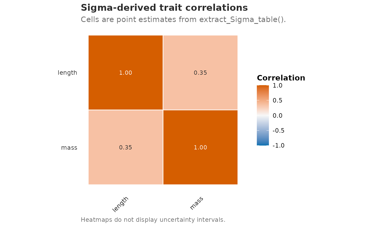
plot_Sigma_heatmap.Rdplot_Sigma_heatmap() turns rows from extract_Sigma_table() into a
matrix-style heatmap. It is designed for articles that need to show the
block structure of a covariance or correlation matrix without manually
extracting Sigma, calling cov2cor(), or rebuilding geom_tile() layers.
Heatmap cells are point estimates only; interval columns, when present, stay
available in the returned plot data but are not displayed.
Usage
plot_Sigma_heatmap(
  x,
  level = "unit",
  part = c("total", "shared", "unique"),
  measure = c("correlation", "covariance"),
  entries = c("all", "unique", "upper", "lower", "offdiag", "diag"),
  link_residual = c("auto", "none"),
  include_diagonal = TRUE,
  facet = c("level", "none"),
  label = TRUE,
  label_digits = 2,
  title = NULL,
  subtitle = NULL,
  caption = NULL
)
Arguments
- x
A fit returned by
gllvmTMB(), an admittedengine = "julia"bridge fit, abootstrap_Sigmaobject, or a data frame returned byextract_Sigma_table(). Data frames must containlevel,trait_i,trait_j,estimate,matrix,component,diagonal, andtriangle;iandjcolumns are used for trait ordering when present.- level, part, measure, entries, link_residual
Passed to
extract_Sigma_table()whenxis a fitted model. The plotting defaultentries = "all"shows the full matrix.- include_diagonal
Logical. Include diagonal rows when present?
- facet
One of
"level"(default) or"none".- label
Logical. Print numeric estimates inside cells?
- label_digits
Number of decimal places for cell labels.
- title, subtitle, caption
Optional scalar character labels.
NULLkeeps the helper's publication-safe defaults.
Details
Scope: the helper plots point-estimate heatmaps from
extract_Sigma_table() rows or extracts those rows from a fit returned by
gllvmTMB(), an admitted engine = "julia" bridge fit, or from a
bootstrap_Sigma object (covered by the package's heatmap validation
tests, which build on the underlying extractor-contract and Julia-bridge
fit tests). It does not display interval bounds or compare fitted values to
known truth. Use plot_Sigma_table() for interval forests or confidence
eyes, and plot_Sigma_comparison() for estimate-vs-truth displays.
vdiffr snapshots and richer multi-model layout helpers remain future figure
work.
Examples
if (requireNamespace("ggplot2", quietly = TRUE)) {
  rows <- data.frame(
    level = "unit",
    trait_i = rep(c("length", "mass"), each = 2),
    trait_j = rep(c("length", "mass"), 2),
    estimate = c(1, 0.35, 0.35, 1),
    matrix = "R",
    component = "total",
    diagonal = c(TRUE, FALSE, FALSE, TRUE),
    triangle = c("diagonal", "lower", "upper", "diagonal")
  )
  plot_Sigma_heatmap(rows)
}