Can I trust this fit?

Before interpreting a fitted GLLVM, separate two questions. Did the optimizer find a numerically healthy point estimate? Does the fitted response distribution show an obvious mismatch to the three behavioural responses arranged in long format? This article answers those questions for a small count example before moving on to covariance, ordination, repeatability, or interval claims.

Use these diagnostics to decide what to inspect or refit next, not as a certificate that every inferential target is calibrated.

The example is deliberately modest: three behaviours counted on each individual, fitted with one shared latent variable. latent() estimates a low-rank axis of between-individual covariance; this is a diagnostic example, not the full ordinary latent() covariance-decomposition tutorial from Morphometrics.

The counts fitted below are Poisson, so nothing here screens the response before fitting. For binary or binomial traits, some conditions are worth checking before you fit at all – rare or constant outcomes, near-duplicate or complementary columns, unusable denominators. screen_gllvmTMB() runs that check; see the pre-fit response screening article for the full walkthrough. Its threshold checks (prevalence, minority counts, duplicate and complement pairs) are advisory: a flag is a hint to inspect the design more closely, not a pass/fail verdict. The optional fixed-design separation module (screen_control(separation = "fixed")) is different in kind – a formal certificate of overlap, complete, or quasi-complete separation over coefficient-connected fixed-design blocks. It does not inspect latent loadings or covariance and does not guarantee convergence; coverage is fixed-design binomial blocks only, and overall screening is partial.

Setup

library(gllvmTMB)
library(ggplot2)

Fit A Small Model

The data have one row per (individual, trait) observation. The working question is whether the three behaviours show a shared between-individual axis and whether the fitted Poisson response model looks reasonable enough to inspect.

set.seed(20260609)

n_ind <- 48L
trait_names <- c("forage", "alarm", "explore")
n_traits <- length(trait_names)

z <- rnorm(n_ind, sd = 0.45)
eta <- cbind(
  forage = 0.25 + 0.75 * z,
  alarm = -0.15 - 0.45 * z,
  explore = 0.05 + 0.55 * z
)
y <- matrix(
  rpois(n_ind * n_traits, lambda = exp(as.vector(eta))),
  nrow = n_ind,
  ncol = n_traits
)

df_long <- data.frame(
  individual = factor(rep(seq_len(n_ind), each = n_traits)),
  trait = factor(rep(trait_names, n_ind), levels = trait_names),
  count = as.vector(t(y))
)

head(df_long, 8)
#>   individual   trait count
#> 1          1  forage     0
#> 2          1   alarm     0
#> 3          1 explore     1
#> 4          2  forage     3
#> 5          2   alarm     0
#> 6          2 explore     0
#> 7          3  forage     1
#> 8          3   alarm     2

The long-format call is canonical. It names the response, the trait column, and the unit column explicitly.

fit_long <- gllvmTMB(
  count ~ 0 + trait +
    latent(0 + trait | individual, d = 1),
  data = df_long,
  trait = "trait",
  unit = "individual",
  family = poisson(),
  control = gllvmTMBcontrol(n_init = 2, init_jitter = 0.03)
)
#> Warning: ! Ordinary `latent()` now includes a per-trait Psi by default (Sigma = Lambda
#>   Lambda^T + Psi).
#> ℹ This changed in gllvmTMB 0.2.0; earlier `latent()` was loadings-only (Lambda
#>   Lambda^T).
#> → Pass `latent(..., unique = FALSE)` for the old rotation-invariant
#>   loadings-only fit.

fit <- fit_long
fit
#> Stacked-trait gllvmTMB fit
#>   Traits = 3, individual = 48 
#>   Covstructs: latent_unit, indep_unit 
#>   Fixed effects (b_fix): 3
#>   ML log L = -190.257   convergence = 0   engine = Laplace
#>   Run gllvmTMB_diagnose(fit) for a full health check, or summary(fit) for parameter estimates.

The same model can be fitted from a wide data frame with the traits(...) left-hand side. The wide call is useful when the data start as one row per individual and one column per behaviour.

df_wide <- stats::reshape(
  df_long,
  idvar = "individual",
  timevar = "trait",
  direction = "wide"
)
names(df_wide) <- sub("^count\\.", "", names(df_wide))

fit_wide <- gllvmTMB(
  traits(forage, alarm, explore) ~ 1 +
    latent(1 | individual, d = 1),
  data = df_wide,
  unit = "individual",
  family = poisson(),
  control = gllvmTMBcontrol(n_init = 2, init_jitter = 0.03)
)

signif(
  abs(as.numeric(logLik(fit_long)) - as.numeric(logLik(fit_wide))),
  3
)
#> [1] 2.14e-09

The observed difference is about 2.14e-09, which is negligible at the reported precision: the two calls reach the same stacked-trait likelihood.

Read Fit Health

The conservative convergence verdict is fit$fit_health$converged. It requires an optimiser success code, a finite objective, and an unscaled maximum gradient below 0.01. scaled_gradient is retained as a descriptive diagnostic, but objective scaling cannot turn a failed optimiser or a large raw gradient into a usable optimum. Hessian curvature and sdreport() remain separate inference checks.

data.frame(
  converged = isTRUE(fit$fit_health$converged),
  optimizer_converged = isTRUE(fit$fit_health$optimizer_converged),
  stationary_by_gradient = isTRUE(fit$fit_health$stationary_by_gradient),
  raw_max_gradient = signif(fit$fit_health$max_gradient, 4),
  raw_gradient_threshold = 0.01,
  scaled_gradient_descriptive = signif(fit$fit_health$scaled_gradient, 4)
)
#>   converged optimizer_converged stationary_by_gradient raw_max_gradient
#> 1      TRUE                TRUE                   TRUE         1.72e-06
#>   raw_gradient_threshold scaled_gradient_descriptive
#> 1                   0.01                   8.995e-09

check_gllvmTMB() returns the detailed, machine-readable fit-health table used in simulations, tests, and reports. gllvmTMB_diagnose() instead prints a guided narrative for an interactive first look. Start with either one before interpreting coefficients, latent variables, or covariance summaries.

health <- check_gllvmTMB(fit)
key_components <- c(
  "optimizer_convergence",
  "max_gradient",
  "sdreport",
  "pd_hessian",
  "weak_axis_unit",
  "boundary_sigma_eps"
)
health[
  health$component %in% key_components,
  c("component", "status", "message")
]
#>                component status
#> 1  optimizer_convergence   PASS
#> 2           max_gradient   PASS
#> 3               sdreport   PASS
#> 4             pd_hessian   WARN
#> 11        weak_axis_unit   PASS
#> 13    boundary_sigma_eps   PASS
#>                                                        message
#> 1                               optimizer reported convergence
#> 2  largest absolute gradient component at the selected optimum
#> 3                                           sdreport available
#> 4      positive-definite Hessian for curvature-based inference
#> 11              Lambda_B column share of shared loading energy
#> 13     sigma_eps is mapped off by the fitted model/family path

These six displayed rows are the headline fit-health checks for this example; read each status column literally (pd_hessian warns here). The full table contains more checks, so always inspect every warning rather than treating a selected subset as the whole verdict. Here are all non-passing rows, including their thresholds, meaning, and suggested action.

health[
  health$status != "PASS",
  c("component", "status", "value", "threshold", "message", "action")
]
#>             component status          value                      threshold
#> 4          pd_hessian   WARN          FALSE                           TRUE
#> 9      boundary_flags   WARN near_zero_sd_B                           none
#> 12 near_zero_psi_unit   WARN       1.03e-07 1e-04 absolute / 0.01 relative
#>                                                                                                     message
#> 4                                                   positive-definite Hessian for curvature-based inference
#> 9                                                      near-boundary loading or variance component detected
#> 12 sd_B minimum fitted per-trait psi standard deviation; collapsed relative to the largest (ratio 0.000476)
#>                                                                                                   action
#> 4                       check gradients, boundary variances, rank, starts, and profile/bootstrap targets
#> 9                                            consider lower rank, simpler covariance, or stronger starts
#> 12 check whether the trait-specific component is intentionally mapped off, boundary-pinned, or redundant

In this fit, the two warnings describe the same feature: the fitted trait-specific diagonal standard deviation is almost zero. The simulation planted a shared latent component without an additional trait-specific between-individual component, so a boundary estimate is plausible here. It still matters for interpretation: this example supports a shared axis, but it does not demonstrate recovery of a separate diagonal variance. “Mapped off” means a parameter was deliberately fixed or excluded from the fitted model, rather than estimated near zero.

Read the rows literally. Optimizer and gradient rows speak to the point estimate. sdreport and pd_hessian speak to Hessian-based standard errors and Wald-style inference. A weak-axis row says a latent variable explains only a small share of the fitted common covariance and may therefore be hard to interpret; it does not by itself prove that the fitted response distribution is wrong.

optimizer_convergence and pd_hessian are worth reading narrowly. The optimizer_convergence row reports only the optimizer’s exit code: it says the optimizer stopped appropriately, not that the point estimate is close to the true generating parameters. (The separate fit$fit_health$converged list field is stricter – it also requires a finite objective and a small maximum gradient – but the same reading applies.) pd_hessian is a local curvature test at that point estimate, not a global check. Read together, a clean table supports “the optimizer stopped appropriately with locally consistent curvature,” not “this fit is near the truth.”

For ordinal_probit() traits, the loading/variance degeneracy screen shown above is binomial-only and does not run on ordinal rows, so a degenerate ordinal fit can pass this table with no warning at all. There is no calibrated ordinal degeneracy detector; see Current limits before treating an ordinal fit as healthy.

boundary_sigma_eps checks the continuous-family residual scale when that parameter is active. A warning means the estimate is below the reported threshold, so the residual scale is close to its boundary; it does not apply when the model or response family maps that parameter off.

The same table records intentionally skipped standard errors. A no-SE fit can still be useful for point estimates or refit-based uncertainty, such as a bootstrap that repeatedly fits the model to new samples, but it should not be reported as if Wald standard errors were computed.

fit_no_se <- gllvmTMB(
  count ~ 0 + trait +
    latent(0 + trait | individual, d = 1),
  data = df_long,
  trait = "trait",
  unit = "individual",
  family = poisson(),
  control = gllvmTMBcontrol(se = FALSE)
)

no_se_health <- check_gllvmTMB(fit_no_se)
no_se_health[
  no_se_health$component %in% c("sdreport", "pd_hessian", "max_fixed_se"),
  c("component", "status", "message")
]
#>      component status
#> 3     sdreport   WARN
#> 4   pd_hessian   WARN
#> 6 max_fixed_se   WARN
#>                                                             message
#> 3 standard-error calculation skipped by gllvmTMBcontrol(se = FALSE)
#> 4           positive-definite Hessian for curvature-based inference
#> 6                               largest fixed-effect standard error

For hard fits, move from this table to the Convergence and start values article before making scientific claims.

When to try `loading_ridge = 2`

Ordinary native Laplace fits stay unpenalised by default, equivalent to loading_ridge = Inf. The control constructor keeps loading_ridge = NULL to preserve that behaviour; it does not impose an infinitely strong penalty. This section concerns ordinary Laplace fits. Opt-in AGHQ has its own aghq_ridge default, described in ?gllvmTMBcontrol.

Try loading_ridge = 2 as a separate sensitivity fit when ordinary between-unit latent loadings become extreme or change substantially between fits. If a Hessian warning remains after checking the data, latent rank and starting values, it is also reasonable to compare this fit, provided a loading prior makes scientific sense. A better Hessian alone is not a reason to choose the result: the prior can supply curvature that the data lack.

The setting puts a zero-mean normal prior with standard deviation 2, variance 4, on free ordinary between-unit loadings. It favours smaller loadings. Smaller positive settings shrink more, while Inf removes the penalty. It does not penalise the trait-specific diagonal covariance or silently extend to spatial, phylogenetic or within-unit loadings. It does not repair separated fixed effects; see When a rare species breaks the JSDM.

What the comparison found

A native-Laplace study fitted 6,000 datasets at each of Inf, 1, 2 and 4: 24,000 attempts in total. It used six traits, two latent axes, estimated trait-specific diagonal covariance and one latent predictor. There were 500 independent datasets per condition: grouped-binomial probit, replicated Gaussian and replicated Poisson, with 100 or 400 units and two loading scales. Failed fits and unavailable intervals stayed in the results.

Loading prior SD	Attempts	Fits with unavailable trait-effect intervals
`Inf`	6,000	64
`1`	6,000	56
`2`	6,000	66
`4`	6,000	62

All optimiser exit codes were zero. The unavailable intervals came from non-positive-definite Hessians, illustrating why that code is insufficient for inference. Ridge 2 restored intervals on 16 datasets relative to Inf but lost them on 18 others. It did not improve availability overall.

Ridge 2 gave modest recovery gains. The largest observed reduction in mean total-covariance error was in the strong-loading binomial condition with 100 units: relative matrix error fell from 0.255 to 0.237. Its paired reduction was 0.0181, with Monte Carlo standard error 0.0021. Trait-effect estimates changed little in the Gaussian conditions.

Coverage means the fraction of repeated datasets whose interval contains the true effect. In the same small-sample binomial condition, the nominal 95% interval for a zero effect covered it in 94.8% of available intervals with Inf, 92.5% with 1, 94.1% with 2 and 94.4% with 4. For a positive effect, coverage was 92.1%, 90.1%, 91.6% and 92.1%, respectively. The coverage estimates have about one percentage point of Monte Carlo uncertainty each. The 2 minus Inf differences in the fractions of all attempts producing an interval containing truth were -0.6 percentage points for the zero effect and -0.4 for the positive effect, with paired Monte Carlo standard errors of about one percentage point. Thus the small differences do not establish a clear coverage improvement or deterioration.

Stronger shrinkage can improve point recovery while narrowing intervals and reducing coverage. The negative effect in the weak-loading Poisson condition with 100 units retained about 91% coverage at every setting. The study does not establish general 95% coverage, and its predictor-informed rank-two results do not certify intercept-only ordination or latent-score intervals. Download the aggregated study tables and fixed-truth data generator for the condition-specific results, uncertainty summaries and provenance. The archive contains aggregate tables, not raw fits or the complete fitting materials.

Compare the same model in either data shape

The following calls use the same data and rank as the earlier example. They illustrate the sensitivity workflow; they do not repeat the coverage study. Keep the original fit alongside the penalised fit.

ridge_control <- gllvmTMBcontrol(
  n_init = 2, init_jitter = 0.03, loading_ridge = 2
)

# Long data: one row per individual and trait.
set.seed(20261018)
fit_ridge_long <- gllvmTMB(
  count ~ 0 + trait + latent(0 + trait | individual, d = 1),
  data = df_long, trait = "trait", unit = "individual",
  family = poisson(), control = ridge_control
)

# Wide data: the same model through traits().
set.seed(20261018)
fit_ridge_wide <- gllvmTMB(
  traits(forage, alarm, explore) ~ 1 + latent(1 | individual, d = 1),
  data = df_wide, unit = "individual",
  family = poisson(), control = ridge_control
)

# Compare trait-scale covariance, which does not depend on axis rotation.
covariance_sensitivity <- lapply(
  list(unpenalised = fit_long, ridge2 = fit_ridge_long),
  extract_Sigma, level = "unit", part = "total", link_residual = "none"
)
lapply(covariance_sensitivity, function(x) round(x$Sigma, 3))
#> $unpenalised
#>         forage  alarm explore
#> forage   0.025  0.019  -0.062
#> alarm    0.019  0.015  -0.048
#> explore -0.062 -0.048   0.154
#> 
#> $ridge2
#>         forage  alarm explore
#> forage   0.024  0.019  -0.059
#> alarm    0.019  0.015  -0.046
#> explore -0.059 -0.046   0.146

# The long and wide ridge fits target the same covariance.
wide_covariance <- extract_Sigma(
  fit_ridge_wide, level = "unit", part = "total", link_residual = "none"
)
signif(max(abs(wide_covariance$Sigma -
               covariance_sensitivity$ridge2$Sigma)), 3)
#> [1] 0
check_gllvmTMB(fit_ridge_long)
#>                   component status                   value
#> 1     optimizer_convergence   PASS                       0
#> 2              max_gradient   PASS               1.618e-06
#> 3                  sdreport   PASS                    TRUE
#> 4                pd_hessian   PASS                    TRUE
#> 5              hessian_rank   PASS                     9/9
#> 6              max_fixed_se   PASS                  0.2069
#> 7           restart_history   PASS                       3
#> 8          selected_restart   PASS                       1
#> 9            boundary_flags   WARN          near_zero_sd_B
#> 10 rotation_convention_unit   PASS as_fit_lower_triangular
#> 11           weak_axis_unit   PASS         min=1; shares=1
#> 12       near_zero_psi_unit   WARN                5.01e-06
#> 13       boundary_sigma_eps   PASS                       1
#>                                                 threshold
#> 1                                                       0
#> 2                                                    0.01
#> 3                                                    TRUE
#> 4                                                    TRUE
#> 5                                               full rank
#> 6                                                     100
#> 7                                                    >= 1
#> 8                                       finite restart id
#> 9                                                    none
#> 10 rotation-invariant Sigma for covariance interpretation
#> 11                                                   0.05
#> 12                         1e-04 absolute / 0.01 relative
#> 13                                                  1e-04
#>                                                        message
#> 1                               optimizer reported convergence
#> 2  largest absolute gradient component at the selected optimum
#> 3                                           sdreport available
#> 4      positive-definite Hessian for curvature-based inference
#> 5  rank of the fixed-parameter covariance matrix from sdreport
#> 6                          largest fixed-effect standard error
#> 7               number of optimizer starts recorded on the fit
#> 8                        restart selected by minimum objective
#> 9         near-boundary loading or variance component detected
#> 10            Lambda_B has an as-fit identification convention
#> 11              Lambda_B column share of shared loading energy
#> 12        sd_B minimum fitted per-trait psi standard deviation
#> 13     sigma_eps is mapped off by the fitted model/family path
#>                                                                                                            action
#> 1                                    try multiple starts, stronger starts, rescaling, or an alternative optimizer
#> 2                                            tighten optimization, rescale predictors, or inspect weak components
#> 3                                           use point summaries cautiously and prefer profile/bootstrap intervals
#> 4                                check gradients, boundary variances, rank, starts, and profile/bootstrap targets
#> 5                                                            treat rank loss as a Hessian/identifiability warning
#> 6                                                 check collinearity, scaling, or weakly identified fixed effects
#> 7                                                            refit with current gllvmTMB if provenance is missing
#> 8                                                         inspect restart_history for competing likelihood basins
#> 9                                                     consider lower rank, simpler covariance, or stronger starts
#> 10 use Sigma/correlations/communality for invariant summaries; rotate or constrain loadings before comparing axes
#> 11                              compare lower ranks, inspect fit stability, and avoid over-interpreting weak axes
#> 12          check whether the trait-specific component is intentionally mapped off, boundary-pinned, or redundant
#> 13                         if estimated near zero, check row-level unique terms or residual-scale identifiability

Inspect whether covariance, fitted means and the effects you intend to report change materially. For a model with lv = ~ x, compare extract_lv_effects(fit, type = "trait_effect"); raw axis coefficients can rotate between fits. If the result is sensitive, report that sensitivity and consider the model structure and prior scale. Comparing 1, 2, 4 and Inf can help; selecting a scale solely because its Hessian passes cannot establish identification or interval calibration.

Finite ridge gives a maximum a posteriori estimate, rather than an ordinary maximum-likelihood estimate. With matching retained curvature metadata, trait-effect intervals are local approximate posterior intervals conditional on the selected prior scale. Unsupported uncertainty remains unavailable. Ordinary AIC, BIC and likelihood-ratio interpretations do not apply to these penalised estimates. The default remains unpenalised.

Check Response Diagnostics

Numerical convergence is not enough. For Gaussian, Poisson, and NB2 rows, residuals(type = "randomized_quantile") evaluates each fitted family’s cumulative distribution function at the observed response. These are exact CDF calculations at the fitted parameter values and fitted random-effect modes, but they do not propagate parameter, refit, or random-effect uncertainty and are not a formal calibration test. NB1 uses the same implemented exact-CDF route and has a display smoke test, but it has not yet reached the same depth of evidence as Gaussian, Poisson, and NB2. diagnostic_table() turns the attached metadata into ordinary data frames for reports and articles.

Family	`type = "randomized_quantile"` result	Status
Gaussian	Exact family-CDF residual	Established
Poisson	Exact family-CDF residual	Established
NB2	Exact family-CDF residual	Established
NB1	Exact family-CDF residual, same route	Implemented, shallower evidence
Every other family	No exact residual: the row is retained with `status = "unsupported_family"` and `residual = NA`; request `type = "simulation_rank"` explicitly for a simulation-based check	Simulation-based route available, not exact
Missing response / non-finite observed value	No residual computed	Row retained with an explicit `status`, never silently dropped

rq <- residuals(
  fit,
  type = "randomized_quantile",
  seed = 20260609
)

diagnostic_table(rq, table = "row_status")
#>   status   n
#> 1     ok 144
diagnostic_table(rq, table = "fit_health_status")
#>   status  n
#> 1   PASS 10
#> 2   WARN  3

head(
  diagnostic_table(rq, table = "data")[
    , c("trait", "family", "observed", "residual", "status")
  ],
  8
)
#>     trait  family observed   residual status
#> 1  forage poisson        0 -1.2801242     ok
#> 2   alarm poisson        0 -0.7317520     ok
#> 3 explore poisson        1  0.4856749     ok
#> 4  forage poisson        3  1.4685245     ok
#> 5   alarm poisson        0 -0.8456795     ok
#> 6 explore poisson        0 -2.1057465     ok
#> 7  forage poisson        1 -0.2994617     ok
#> 8   alarm poisson        2  0.6812327     ok

The row_status table tells you whether every model row produced a usable residual. If a row is marked unsupported_family, missing_response, or nonfinite_observed, keep that status in the report rather than silently dropping the row.

The Q-Q points below stay broadly near the reference line through the centre, but the alarm and forage panels depart in the upper tail. The display is useful because it does not turn a mostly straight pattern into a blanket pass: those tails deserve inspection, and the plot is not evidence that the latent rank or uncertainty estimates are calibrated.

predictive_check(
  fit,
  type = "rq_qq",
  seed = 20260609
)

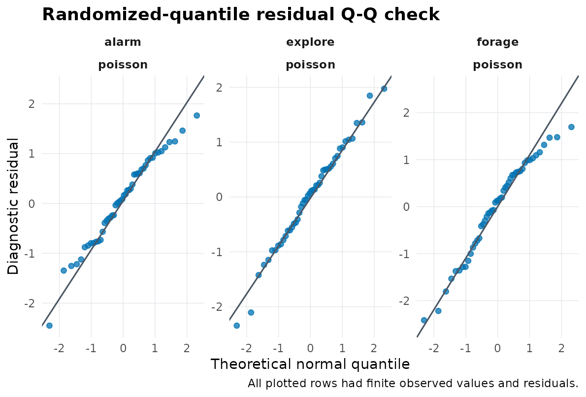
Randomized-quantile residual Q-Q check for the fitted Poisson GLLVM. This is a fitted-model diagnostic display, not interval calibration, latent-rank proof, or a Bayesian posterior predictive check.

For Poisson and NB2 count models, a rootogram is often easier to read than a Q-Q plot. Bars near zero mean the observed and fitted-model simulated count frequencies are similar on the square-root scale. The simulations default to condition_on_RE = TRUE, so they condition on the fitted random-effect modes; they check the fitted response pattern, not the marginal random-effect distribution. The plot below shows noticeable alternating discrepancies, especially for forage counts 3 and 5. They do not all point in one direction, but they are large enough to investigate rather than dismiss. Simulation noise remains, even with the larger draw count used here.

predictive_check(
  fit,
  type = "rootogram",
  ndraws = 200,
  seed = 20260609,
  max_count = 7L
)

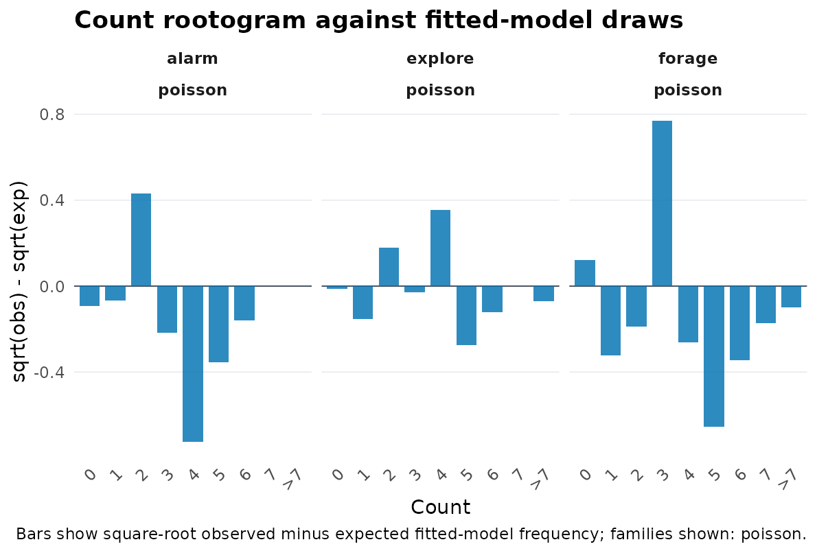
Rootogram comparing observed behavioural counts with simulations conditional on the fitted random-effect modes. Persistent departures can flag a response-family, link, covariate, offset, or fitted-linear-predictor mismatch; this display does not test the marginal random-effect distribution.

Coming From DHARMa

If DHARMa is your reference point from glmmTMB workflows, the rough correspondence is: DHARMa’s simulation-based residuals map to residuals(fit, type = "simulation_rank"), and DHARMa’s diagnostic plots map to predictive_check(fit, ...). This is a conceptual mapping, not DHARMa compatibility – gllvmTMB does not wrap or reproduce DHARMa, and it does not currently provide DHARMa’s formal uniformity, dispersion, or outlier tests. Never treat the two as equivalent. Predictive plots here are diagnostic display only: no interval calibration, latent-rank proof, or DHARMa-equivalent formal test.

What To Do Next

Use the diagnostics as routing information, not as a single pass/fail stamp.

What you see	What it means	Next step
The four numerical rows shown above all pass	The numerical fit is a reasonable starting point, provided the remaining rows contain no unexplained warnings	Inspect every non-PASS row, then inspect `Sigma`, correlations, ordination, or fitted effects.
Optimizer or gradient rows warn/fail	The point estimate may be unstable	Try more starts, rescaling, simpler rank, or an alternative optimizer.
`sdreport` or `pd_hessian` warns	Wald uncertainty is unavailable or local curvature may be unreliable	Inspect the scientific target and use a supported profile or refit-based bootstrap route where available.
Residual rows have non-`ok` status	Some rows were not diagnosed	Inspect missing values, non-finite responses, and family support.
Q-Q or rootogram shows systematic structure	The fitted conditional response pattern may be wrong	Revisit family, link, covariates, offsets, or the fitted linear predictor; investigate random effects separately.

If the fit-health and response checks are acceptable but the latent rank is still a modelling choice, continue to How many latent dimensions should I fit?. That article compares one ML candidate set with AIC/BIC and uses REML only after a Gaussian model has been chosen.

What A Simulation Check Can Establish

Simulation is useful only when its question is named. Three common checks answer different questions:

Check	What it can show	What it cannot show
Fitted-model predictive draw	Selected response patterns	Biological truth, latent rank, or interval calibration
Fitted-model simulate–refit	Local pipeline self-consistency	Real-data truth or protection against misspecification
Predeclared known-DGP grid	Bias, recovery, and interval performance in the studied regime	Performance outside the regimes actually studied

One simulated dataset is an illustration, not recovery evidence. A validation study needs repeated independent datasets, an estimand that matches the fitted model, and separate counts for attempted fits, healthy fits, usable intervals, and successful coverage. It should also report Monte Carlo uncertainty rather than turning a small number of replicates into a pass/fail certificate.

This page covers fit health and no-SE status, fitted-model predictive diagnostics and residuals for Gaussian, Poisson, and NB2 rows, and report-ready metadata tables. NB1 uses an implemented exact-CDF route, but its evidence is currently shallower than for those three families.

The page does not calibrate confidence intervals, prove the latent rank, run formal residual tests, test the marginal random-effect distribution, or draw from a Bayesian posterior. Exact residual support for delta, hurdle, truncated, ordinal, and mixture-family rows remains outside its current claims.