
Integrating opportunistic records with a designed survey: a small worked example
Source:vignettes/articles/integrated-two-source-example.Rmd
integrated-two-source-example.RmdExperimental. The model here is fitted through the ordinary
gllvmTMB()entry point — there is no separate integrated-model function — but the route is experimental: the interface may change without deprecation, and no released capability claim is made. The example exists so that early users can see the intended workflow end to end on simulated data.
The question
Opportunistic portal records (GBIF-style) are abundant but arrive where people go; a designed detection/non-detection survey is small but has known effort. This example asks a deliberately modest question of a simulated three-species grassland songbird guild on a prairie-inspired landscape: after giving the portal records their own recording-bias term, do the two sources agree on one shared habitat gradient?
Both sources see the same ecological state for species in cell ,
with
a measured habitat covariate and
an unmeasured shared spatial gradient carried by a latent field with
species loadings
.
The portal branch adds what only it suffers – a per-species reporting
level
,
an accessibility bias with species-specific coefficients
,
and its own spatial recording field – while the survey branch is a plain
complementary-log-log (cloglog) detection/non-detection
likelihood with known visit support:
The
term (fitted below as trait:isdm_gbif) is not decoration:
it is the identification device this model class requires. Presence-only
records cannot say how many records “should” occur per unit
intensity, only where relatively more occur. Without a per-species
reporting level on the presence-only arm, the two arms would share an
absolute intercept and the fit would implicitly claim the absolute
intensity that presence-only data cannot identify.
Everything is relative intensity: no absolute abundance, occupancy, or detectability claim is available from this design.
This is the intrinsic shape of the problem, not a stylistic choice:
the per-row family selector below needs several observation rows per
(cell, species) that carry different response families, which
is exactly what the long-format grammar represents and the wide
traits() grammar cannot – a wide row is one (cell, species)
cell with one family. There is no wide version of this example to show
alongside it.
Simulate a small two-source data set
One hundred and eight cells, three species, one portal record stream, three survey visits. The fields here are simple smooth surfaces that let you see how the model works; this one simulated dataset cannot establish recovery accuracy.
n_lon <- 12; n_lat <- 9
grid <- expand.grid(lon = seq(0, 1.2, length.out = n_lon),
                    lat = seq(0, 0.9, length.out = n_lat))
grid <- grid[order(grid$lat, grid$lon), ]
n_cell <- nrow(grid)
cells   <- paste0("cell_", seq_len(n_cell))
species <- c("gralark", "dickcis", "bobolnk")   # simulated guild

## habitat covariate, shared gradient u, and an accessibility index
x <- as.numeric(scale(grid$lon))                        # measured habitat
u <- 0.8 * sin(pi * grid$lat / 0.9) * cos(pi * grid$lon / 1.2)  # unmeasured
b <- as.numeric(scale(-grid$lat + 0.3 * cos(2 * pi * grid$lon)))# access bias
## the DGP here has NO portal-only spatial field (delta = 0): the fitted
## model still estimates one, and treating it as a nuisance is the honest
## reading at this design size (see the closing cautions)

alpha  <- c(-0.3, 0.1, 0.4)
beta   <- c(0.6, -0.4, 0.5)
lambda <- c(0.9, 0.7, -0.6)
gamma  <- c(0.5, -0.3, 0.2)

eta <- outer(u, lambda) +
  sweep(outer(x, beta), 2, alpha, "+")                  # n_cell x 3

## portal effort concentrates in accessible cells; survey support is designed
a_g <- 3 * exp(0.4 * b + rnorm(n_cell, sd = 0.2))
a_s <- rep(0.9, n_cell)

base <- expand.grid(cell_id = cells, trait = species,
                    stringsAsFactors = FALSE)
base <- base[order(match(base$cell_id, cells), match(base$trait, species)), ]
ci <- match(base$cell_id, cells)
si <- match(base$trait, species)

gbif <- transform(base, source = "gbif", survey_event_id = NA_character_,
  branch = "count", support = a_g[ci], lon = grid$lon[ci], lat = grid$lat[ci],
  value = rpois(nrow(base),
    a_g[ci] * exp(eta[cbind(ci, si)] + b[ci] * gamma[si])),
  visit = NA_integer_)

pa <- do.call(rbind, lapply(1:3, function(v) transform(base,
  source = "survey", survey_event_id = paste0("pa_v", v, "_", base$cell_id),
  branch = "pa", support = a_s[ci], lon = grid$lon[ci], lat = grid$lat[ci],
  value = rbinom(nrow(base), 1, -expm1(-a_s[ci] * exp(eta[cbind(ci, si)]))),
  visit = v)))

rows <- rbind(gbif, pa)
table(rows$source)
#>
#>   gbif survey
#>    324    972
The shared gradient u is what both sources are supposed
to see in common. Mapping it over the grid before fitting anything gives
a visual reference for the “do the two sources agree?” question the rest
of the article works toward:
ggplot(grid, aes(lon, lat, fill = u)) +
  geom_raster() +
  scale_fill_gradient2(low = "#8c4d8f", mid = "white", high = "#0a617d") +
  coord_fixed() +
  labs(x = "Longitude (arbitrary units)", y = "Latitude (arbitrary units)",
       fill = "Shared gradient (u)") +
  theme_minimal()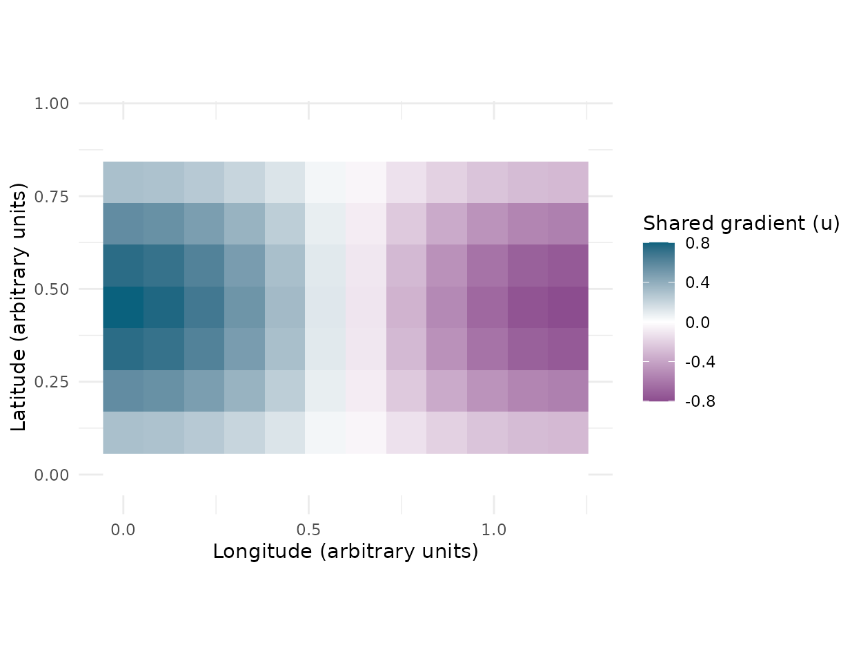
The simulated shared spatial gradient u across the 108-cell grid. Both the portal stream and the survey observe species intensities driven partly by this common field; neither source sees u directly.
Assemble the long table
gllvmTMB() works on long data: one row per (cell,
species, source). Three columns do the work that makes this an
integrated model rather than two models glued together.
dat <- rows
dat$trait   <- factor(dat$trait)
dat$cell_id <- factor(dat$cell_id)

## 1. the portal-row indicator: 1 on portal rows, 0 on survey rows. Every portal-only
##    term is written as an interaction with this, so it is structurally
##    absent from the survey likelihood rather than merely small.
dat$isdm_gbif <- as.integer(dat$source == "gbif")

## 2. known support, on the log scale: portal effort and survey visit area.
##    This is the change-of-support term, not a parameter.
dat$log_support <- log(dat$support)

## 3. the covariates. `bias` is portal-only, so it is a structural zero on
##    survey rows -- a zero, never an NA, because a survey row genuinely has
##    no accessibility term rather than a missing one.
dat$env  <- x[match(as.character(dat$cell_id), cells)]
dat$bias <- ifelse(dat$isdm_gbif == 1L,
                   b[match(as.character(dat$cell_id), cells)], 0)

## the per-row family selector, and the family list it selects from
dat$isdm_family <- factor(ifelse(dat$source == "gbif", "gbif", "survey_pa"),
                          levels = c("gbif", "survey_pa"))
fam <- list(gbif = poisson(), survey_pa = binomial(link = "cloglog"))
attr(fam, "family_var") <- "isdm_family"
The family list is the heart of it. Ordinarily
gllvmTMB() requires one family per trait; here a single
species is Poisson on its portal rows and Bernoulli-cloglog on its
survey rows. That mix is admitted because cloglog is the link under
which a detection/non-detection observation is mathematically consistent
with the same underlying intensity that generates the Poisson counts –
not an approximation. It also works because neither Poisson nor
Bernoulli carries a dispersion (overdispersion) parameter, so there is
no ambiguity about which family owns a per-species dispersion.
The contract is exact, not approximate. Mixing
families within a trait is admitted only for
family = list(gbif = poisson(), survey_pa = binomial(link = "cloglog"))
(Poisson-log paired with binomial-cloglog), together with a
family_var attribute naming the per-row selector column and
a matching factor column in the data. Anything short of that falls back
to the ordinary one-family-per-trait rule and errors there, because from
the fitter’s point of view it no longer looks like an integrated fit at
all. The three ways to fall short:
- a missing or misnamed
family_varattribute; - a
sourcecolumn present without its matchingisdm_familylevels; - only one of the two sources actually present in the data.
Swapping the survey link for logit or probit is refused outright: those links do not share the intensity that generates the portal counts, so the two branches would no longer describe the same .
Fit the integrated model
The two sources enter one likelihood: shared fixed effects and shared
latent field, a portal-only bias coefficient and portal-only spatial
field, and the survey’s cloglog detection branch – selected per row by
isdm_family. A mesh over the cells carries the spatial
terms.
mesh <- make_mesh(dat[, c("lon", "lat")], c("lon", "lat"), cutoff = 0.085)
fit <- gllvmTMB(
  value ~ 0 + trait + trait:env + trait:isdm_gbif + trait:bias +
    offset(log_support) +
    indep(0 + trait | cell_id) +
    spatial_latent(1 + isdm_gbif | cell_id, d = 1),
  data   = dat,
  trait  = "trait",
  unit   = "cell_id",
  family = fam,
  mesh   = mesh,
  silent = TRUE
)
That one call has now estimated the shared slopes, the portal’s reporting level and bias terms, both spatial fields, and the survey’s cloglog branch, all from one likelihood. Before reading any coefficient, check whether the fit is trustworthy — starting with the mesh both spatial terms rest on:
plot(mesh)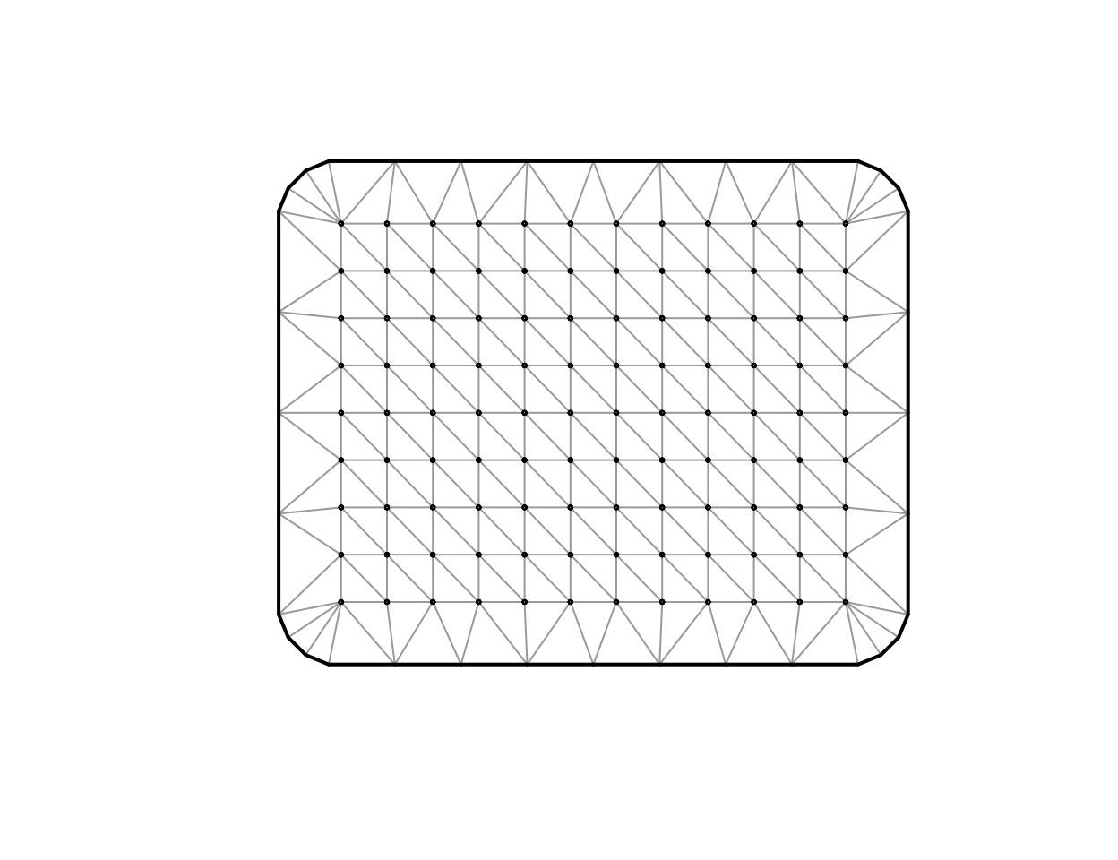
Triangular SPDE mesh built from the 108 grid cells. The mesh carries both the shared spatial field u and the portal-only recording field at its vertices; the observation-to-mesh projection maps each back to the cell rows fitted above.
Did the fit converge, and can you trust its curvature?
fit$opt$convergence
#> [1] 0
0 is the optimizer’s own signal that it stopped at a
point it judges stationary – not proof that the point is a good
estimate, and not a substitute for checking curvature.
check_gllvmTMB() runs that second, independent check: it
reports whether the Hessian at the optimum is positive-definite, which
is what actually licenses Wald-type standard errors.
health <- check_gllvmTMB(fit)
health[
  health$component %in% c("optimizer_convergence", "pd_hessian"),
  c("component", "status", "value")
]
#>               component status value
#> 1 optimizer_convergence   PASS     0
#> 4            pd_hessian   PASS  TRUE
optimizer_convergence reads PASS: the
optimizer itself is content. But pd_hessian reads
WARN – the Hessian at this optimum is not
positive-definite. That combination (stationary point, non-PD curvature)
is consistent with the first caution below: source-specific spatial
structure is only weakly identified at this design size, and a weakly
identified spatial covariance is exactly the kind of thing that leaves
the Hessian non-PD even while the optimizer is satisfied.
It is worth being precise about which part of the model is
responsible, because it is not the integration. Refitting these same
data with the spatial terms replaced by an ordinary non-spatial
latent() block – same two sources, same shared predictor,
same portal-bias coefficient – returns pd_hessian = PASS.
The integrated likelihood is not the difficulty; the spatial
fields are, at 108 cells. That is the same conclusion the design
article reaches from a much larger set of fits, and it is why the
companion How big does an
integrated survey design need to be? exists.
Read this as the honest state of a small illustrative fit, not as a
bug – but do not trust Wald-type standard errors from this particular
fit, and do not skip this check on your own data because a real analysis
is unlikely to be this forgiving. See Convergence and start values
for the fuller triage (more starts, rescaling, a simpler covariance)
when pd_hessian warns on a fit you intend to use.
What did the two sources agree on?
The portal-bias coefficients are the part of the model only the integration can give you – the survey anchors the shared state, so is identified rather than silently absorbed. At this deliberately small design expect useful but noisy estimates:
## factor() ordered the species alphabetically, so the fitted coefficients come
## back in that order -- realign the simulated truth before comparing, and name
## the columns so the pairing is visible rather than assumed.
idx <- grep("bias", fit$X_fix_names)
gamma_ordered <- gamma[match(levels(dat$trait), species)]
tab <- rbind(truth = gamma_ordered, estimate = unname(fit$opt$par[idx]))
colnames(tab) <- levels(dat$trait)
round(tab, 2)
#>          bobolnk dickcis gralark
#> truth       0.20   -0.30    0.50
#> estimate    0.16   -0.34    0.48
gamma_df <- data.frame(
  species  = levels(dat$trait),
  truth    = gamma_ordered,
  estimate = unname(fit$opt$par[idx])
)
lims <- range(c(gamma_df$truth, gamma_df$estimate)) + c(-0.1, 0.1)
ggplot(gamma_df, aes(truth, estimate, label = species)) +
  geom_abline(slope = 1, intercept = 0, colour = "grey55", linewidth = 0.5) +
  geom_point(size = 2.8, colour = "#0a617d") +
  geom_text(vjust = -1, size = 3.3) +
  coord_equal(xlim = lims, ylim = lims) +
  labs(x = "True gamma", y = "Fitted gamma") +
  theme_minimal()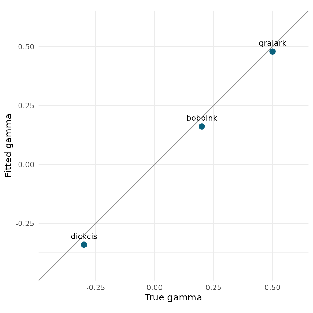
True versus fitted portal accessibility-bias coefficients gamma, one point per species. The line marks exact recovery; distance from it is recovery error at this design size.
All three species land close to the identity line on this draw: the
portal-only bias term separates recording effort from the shared
ecological signal rather than absorbing it into
or
.
bobolnk (the smallest true
)
is the noisiest of the three in relative terms, which is the expected
pattern: a near-zero true effect is the hardest one to pin down
precisely, not evidence that the method singles that species out.
The shared-state loadings and the portal-only field’s covariance are
reported on the link scale (both are sign-invariant as outer products).
Use extract_Sigma() to attach trait names and check that
the fit contains this covariance term:
sigma_slope <- extract_Sigma(fit, level = "spde_slope")
round(sigma_slope$intercept, 3)
#>         bobolnk dickcis gralark
#> bobolnk   6.182  -4.851  -8.401
#> dickcis  -4.851   3.807   6.593
#> gralark  -8.401   6.593  11.418
round(sigma_slope$slope, 3)
#>         bobolnk dickcis gralark
#> bobolnk   1.180  -0.664  -4.094
#> dickcis  -0.664   0.373   2.302
#> gralark  -4.094   2.302  14.198
sigma_slope$intercept is the shared spatial field’s
cross-species covariance: it is what carries the “one shared gradient”
question, and its sign pattern should echo the simulated loadings
lambda above (gralark and dickcis
positively coupled, bobolnk moving the other way).
sigma_slope$slope is the portal-only field’s covariance –
here it is estimating structure that the data-generating process never
put there (delta = 0 above), so its magnitude is a measure
of how much unclaimed spatial variance the portal branch is willing to
soak up at this design size, not a recovered effect to interpret species
by species. Reading it alongside the first caution below is deliberate:
this is exactly the quantity that caution says to treat as a nuisance
adjustment.
What to check before believing more than this
Three honest cautions, each with a package-level reason.
- Design size governs identifiability. Source-specific spatial structure is only weakly identified on small grids: simulations with known parameter values place reliable recovery of a portal-only field far beyond a design of this size, with identifiability bought by adding cells (at maintained per-cell records), not by piling records into the same cells. Treat the portal-only field here as a nuisance adjustment, not an estimate to interpret.
- Relative intensity only. Nothing in this design identifies absolute abundance or detectability; comparisons are within-map, not across species in absolute terms. And the bias coefficients carry their own design requirement: the accessibility covariate must vary separately from the habitat covariate (and from the portal-only spatial field), or bias and ecology are confounded and no fitting choice can separate them. The simulation satisfies this by construction; in real data it is yours to check.
- Experimental surface. The route is public but experimental: the data contract and the terms above may change without deprecation. Check convergence and positive-definiteness on every fit, and do not build a pipeline on this interface yet.
What this route does and does not cover
Covered here: two sources — one presence-only count
stream and one detection/non-detection survey — sharing one ecological
linear predictor, with a portal-only bias term and known per-row
support, fitted through gllvmTMB().
Accuracy remains uncertain: the model fits this example, but recovery accuracy at this or any particular design size is not established. In particular, no completed recovery study establishes the accuracy of the portal-only spatial field. Read the numbers above as an illustration of the workflow, not evidence of reliable parameter recovery.
Not available: more than two sources through
this article’s manual two-source contract — for any number of named
sources, use the isdm_sources() declaration shown in More than two sources;
calibrated confidence intervals for this route; and weighting one
source’s contribution against the other’s. The latter two are real work,
not an oversight.
See also
-
Multivariate spatial models with an
SPDE mesh for
spatial_latent()and mesh construction on their own, outside the two-source setting. - Choose a response family for the ordinary one-family-per-trait rule that this article’s per-row contract is an exception to.
References
Fithian, W., Elith, J., Hastie, T. and Keith, D.A. (2015). Bias correction in species distribution models: pooling survey and collection data for multiple species. Methods in Ecology and Evolution 6, 424–438. https://doi.org/10.1111/2041-210X.12242
Fletcher, R.J. Jr, Hefley, T.J., Robertson, E.P., Zuckerberg, B., McCleery, R.A. and Dorazio, R.M. (2019). A practical guide for combining data to model species distributions. Ecology 100, e02710. https://doi.org/10.1002/ecy.2710
Isaac, N.J.B., Jarzyna, M.A., Keil, P., et al. (2020). Data integration for large-scale models of species distributions. Trends in Ecology & Evolution 35, 56–67. https://doi.org/10.1016/j.tree.2019.08.006
Koshkina, V., Wang, Y., Gordon, A., Dorazio, R.M., White, M. and Stone, L. (2017). Integrated species distribution models: combining presence-background data and site-occupancy data with imperfect detection. Methods in Ecology and Evolution 8, 420–430. https://doi.org/10.1111/2041-210X.12738
Miller, D.A.W., Pacifici, K., Sanderlin, J.S. and Reich, B.J. (2019). The recent past and promising future for data integration methods to estimate species’ distributions. Methods in Ecology and Evolution 10, 22–37. https://doi.org/10.1111/2041-210X.13110