Behavioural syndromes in repeated measurements • gllvmTMB

Evidence boundary. This article demonstrates point estimation for one Gaussian repeated-measures model. It does not establish confidence-interval calibration.

A behavioural syndrome is stable covariance among behaviours at the individual level. Repeated measurements also contain covariance among behaviours within an individual from one occasion to another. Those are different biological summaries:

Between individuals: do consistently bolder individuals also tend to be more exploratory or active?
Within individuals: when an individual’s measurement departs from its usual level on one occasion, do several behaviours depart together?

This article separates those two covariance matrices and computes trait-specific repeatability. The within-occasion component can combine short-term state, unmeasured context, and measurement error; the model does not identify which of those mechanisms caused it.

The model

For individual $i$ , occasion $s$ , and trait $t$ , we fit

$y_{ist} = \mu_t + b_{it} + w_{ist}.$

$\mathbf b_i \sim \operatorname{MVN}(0, \Sigma_B), \qquad \mathbf w_{is} \sim \operatorname{MVN}(0, \Sigma_W).$

Each covariance uses a low-rank shared component plus a trait-specific diagonal:

$\Sigma_B = \Lambda_B\Lambda_B^\top + \Psi_B, \qquad \Sigma_W = \Lambda_W\Lambda_W^\top + \Psi_W.$

The per-trait repeatability, or intraclass correlation, is

$R_t = \frac{(\Sigma_B)_{tt}} {(\Sigma_B)_{tt} + (\Sigma_W)_{tt}}.$

Target	Formula term	Interpretation
$\Sigma_B$	`latent(... \\| individual)`	Stable covariance among individual means
$\Sigma_W$	`latent(... \\| occasion)`	Covariance among occasion-level deviations, including inseparable measurement error
$R_t$	both tiers	Proportion of fitted variance that lies between individuals for trait $t$

Repeatability is not heritability: stable genetic and environmental differences both contribute to $\Sigma_B$ . This model is also not a reaction norm. A reaction norm includes a measured environmental gradient and asks whether individuals differ in their slopes along it.

Data requirements

The example uses standardized continuous traits and a Gaussian likelihood. Before fitting real data:

Give every measurement occasion a unique identifier nested within individual. Reusing occasion = 1, 2, ... across individuals would join unrelated observations into the same random-effect level.
Confirm that individuals have repeated occasions. Uneven replication is allowed, but individuals with little information contribute little to the between/within separation.
Check that each (individual, occasion, trait) cell represents the intended observation. Resolve accidental duplicates before fitting.
Put continuous traits on interpretable, comparable scales when their raw units differ greatly. Counts, proportions, and ordinal scores need likelihoods appropriate to their sampling process rather than automatic Gaussian treatment.
Choose the two ranks deliberately. This teaching simulation plants $d_B=2$ and $d_W=1$ ; it does not estimate those ranks.

See Choosing latent rank for rank sensitivity and Handling missing data when the repeated trait grid is incomplete.

Simulate a truth-checked example

library(gllvmTMB)

We simulate six behaviours for 150 individuals measured on six occasions. The between-individual tier has two anonymous latent axes; the occasion tier has one. We do not attach biological names to raw latent axes because their orientation and sign are not identified without an explicit rotation or constraint.

set.seed(2025)
n_individual <- 150L
n_occasion <- 6L
trait_names <- c(
  "boldness", "exploration", "latency_emerge",
  "aggression", "activity", "restlessness"
)
n_traits <- length(trait_names)

Lambda_B_true <- matrix(
  c(
     0.55, 0.00,
     0.45, 0.05,
    -0.40, 0.00,
     0.05, 0.55,
     0.05, 0.45,
     0.00, 0.35
  ),
  n_traits,
  2,
  byrow = TRUE,
  dimnames = list(trait_names, c("B1", "B2"))
)
psi_B_true <- setNames(rep(0.10, n_traits), trait_names)

Lambda_W_true <- matrix(
  c(0.25, 0.20, -0.18, 0.22, 0.20, 0.18),
  n_traits,
  1,
  dimnames = list(trait_names, "W1")
)
# This diagonal includes unshared occasion variation and measurement error.
psi_W_true <- setNames(rep(0.35, n_traits), trait_names)

Sigma_B_true <- tcrossprod(Lambda_B_true) + diag(psi_B_true)
Sigma_W_true <- tcrossprod(Lambda_W_true) + diag(psi_W_true)
R_true <- diag(Sigma_B_true) /
  (diag(Sigma_B_true) + diag(Sigma_W_true))

between <- matrix(rnorm(n_individual * 2), n_individual, 2) %*%
  t(Lambda_B_true) +
  sweep(
    matrix(rnorm(n_individual * n_traits), n_individual, n_traits),
    2,
    sqrt(psi_B_true),
    "*"
  )

n_rows_wide <- n_individual * n_occasion
individual_index <- rep(seq_len(n_individual), each = n_occasion)
within <- matrix(rnorm(n_rows_wide), n_rows_wide, 1) %*%
  t(Lambda_W_true) +
  sweep(
    matrix(rnorm(n_rows_wide * n_traits), n_rows_wide, n_traits),
    2,
    sqrt(psi_W_true),
    "*"
  )
Y <- between[individual_index, ] + within

df_wide <- data.frame(
  individual = factor(individual_index),
  occasion = factor(paste(
    individual_index,
    rep(seq_len(n_occasion), n_individual),
    sep = "_"
  ))
)
df_wide[trait_names] <- as.data.frame(Y)

df_long <- data.frame(
  individual = factor(rep(individual_index, n_traits)),
  occasion = factor(rep(df_wide$occasion, n_traits)),
  trait = factor(
    rep(trait_names, each = n_rows_wide),
    levels = trait_names
  ),
  value = as.vector(Y)
)

stopifnot(
  !anyDuplicated(df_long[c("individual", "occasion", "trait")]),
  all(table(df_long$individual) == n_occasion * n_traits),
  all(table(df_long$occasion) == n_traits)
)
head(df_long)
#>   individual occasion    trait      value
#> 1          1      1_1 boldness  0.6145134
#> 2          1      1_2 boldness  1.1313808
#> 3          1      1_3 boldness  0.9165687
#> 4          1      1_4 boldness  0.4907240
#> 5          1      1_5 boldness  1.5877557
#> 6          1      1_6 boldness -0.8902190

The example puts all unshared occasion-level variation, including measurement error, inside $\Psi_W$ . That matches what this data resolution can identify; it does not pretend to estimate a separate measurement-error variance.

Fit long and wide forms

The long form has one row per individual-occasion-trait observation. The wide form has one row per individual occasion and one response column per trait. Both use the same gllvmTMB() entry point.

fit_control <- gllvmTMBcontrol(
  start_method = list(method = "indep"),
  optimizer = "optim",
  optArgs = list(method = "BFGS")
)

fit_long <- gllvmTMB(
  value ~ 0 + trait +
    latent(0 + trait | individual, d = 2, unique = TRUE) +
    latent(0 + trait | occasion, d = 1, unique = TRUE),
  data = df_long,
  trait = "trait",
  unit = "individual",
  unit_obs = "occasion",
  family = gaussian(),
  control = fit_control
)

fit_wide <- gllvmTMB(
  traits(
    boldness, exploration, latency_emerge,
    aggression, activity, restlessness
  ) ~ 1 +
    latent(1 | individual, d = 2, unique = TRUE) +
    latent(1 | occasion, d = 1, unique = TRUE),
  data = df_wide,
  unit = "individual",
  unit_obs = "occasion",
  family = gaussian(),
  control = fit_control
)

c(
  long = as.numeric(logLik(fit_long)),
  wide = as.numeric(logLik(fit_wide)),
  absolute_difference = abs(
    as.numeric(logLik(fit_long)) - as.numeric(logLik(fit_wide))
  )
)
#>                long                wide absolute_difference 
#>       -5.750598e+03       -5.750598e+03        1.412332e-06

The two likelihoods should agree up to numerical precision. This verifies the data-shape translation, not two independent scientific analyses.

Inspect every numerical warning

health <- check_gllvmTMB(fit_long)

data.frame(
  converged = isTRUE(fit_long$fit_health$converged),
  raw_max_gradient = signif(fit_long$fit_health$max_gradient, 4),
  raw_gradient_threshold = 0.01,
  scaled_gradient_descriptive = signif(
    fit_long$fit_health$scaled_gradient,
    4
  )
)
#>   converged raw_max_gradient raw_gradient_threshold scaled_gradient_descriptive
#> 1      TRUE         0.001333                   0.01                   2.318e-07

core_components <- c(
  "optimizer_convergence",
  "max_gradient",
  "sdreport",
  "pd_hessian"
)

health[
  health$component %in% core_components,
  c("component", "status", "message")
]
#>               component status
#> 1 optimizer_convergence   PASS
#> 2          max_gradient   PASS
#> 3              sdreport   PASS
#> 4            pd_hessian   PASS
#>                                                       message
#> 1                              optimizer reported convergence
#> 2 largest absolute gradient component at the selected optimum
#> 3                                          sdreport available
#> 4     positive-definite Hessian for curvature-based inference

stopifnot(
  isTRUE(fit_long$fit_health$converged),
  all(health$status[health$component %in% core_components] == "PASS")
)

health[
  health$status != "PASS",
  c("component", "status", "value", "threshold", "message", "action")
]
#>                   component status              value
#> 10 rotation_convention_unit   WARN rotation_ambiguous
#>                                                 threshold
#> 10 rotation-invariant Sigma for covariance interpretation
#>                                                  message
#> 10 Lambda_B is identified up to rotation/sign convention
#>                                                                                                            action
#> 10 use Sigma/correlations/communality for invariant summaries; rotate or constrain loadings before comparing axes

The rendered BFGS fixture passes the optimiser and raw-gradient checks, so its point covariance is numerically usable. The sdreport() and Hessian rows also pass, which supports local Wald calculations. Keep those decisions separate: an optimiser failure or raw maximum gradient above 0.01 challenges the point surface, whereas an sdreport() or Hessian warning blocks or weakens Wald inference without automatically invalidating a stable rotation-invariant point covariance. The objective-scaled gradient is descriptive and cannot override a failed optimiser or large raw gradient. Matching long/wide likelihoods checks data-shape translation only; it does not establish interval coverage.

The rotation warning concerns the raw between-individual loading matrix. It does not invalidate the rotation-invariant covariance $\Sigma_B$ , but it does mean that unrotated labels such as “LV1 = boldness” are unsafe.

Recover both covariance tiers

Sigma_B_hat <- extract_Sigma(
  fit_long,
  level = "unit",
  part = "total"
)$Sigma
Sigma_W_hat <- extract_Sigma(
  fit_long,
  level = "unit_obs",
  part = "total"
)$Sigma

relative_error <- c(
  between = norm(Sigma_B_hat - Sigma_B_true, "F") /
    norm(Sigma_B_true, "F"),
  within = norm(Sigma_W_hat - Sigma_W_true, "F") /
    norm(Sigma_W_true, "F")
)
round(relative_error, 3)
#> between  within 
#>   0.173   0.094

These are descriptive errors for one simulated dataset. They check that the worked example recovers its two scientific targets; they are not a repeated-sampling validation study.

between_comparison <- compare_Sigma_table(
  fit_long,
  truth = Sigma_B_true,
  level = "unit",
  measure = "correlation",
  entries = "upper"
)
between_comparison$comparison <- "Between individuals"

within_comparison <- compare_Sigma_table(
  fit_long,
  truth = Sigma_W_true,
  level = "unit_obs",
  measure = "correlation",
  entries = "upper"
)
within_comparison$comparison <- "Within individuals"

covariance_comparison <- rbind(
  between_comparison,
  within_comparison
)

plot_Sigma_comparison(
  covariance_comparison,
  measure = "correlation",
  facet = "comparison",
  style = "scatter"
)

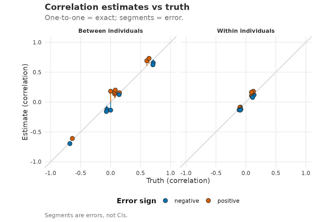
Two scatterplot panels compare fitted with true correlations among six behaviours. One panel shows stable between-individual correlations and the other shows within-individual occasion correlations. A diagonal line in each panel marks exact recovery.

Fitted versus true trait correlations at the between-individual and within-individual tiers. The diagonal line marks exact recovery; points are estimates, not confidence intervals.

The plotted targets are the total covariance matrices. The simulation also has shared and diagonal pieces, but this single fit does not justify a biological interpretation of their exact split. In real data, interpret total between/within covariance first and treat loading or communality stories as rank- and rotation-dependent.

Recover repeatability

extract_repeatability() uses the Wald route by default. We display only its point estimate because this article does not establish interval calibration. A request for method = "profile" stops rather than silently substituting a Wald interval; use method = "bootstrap" only when its refit-based limitations are appropriate for the analysis.

repeatability <- extract_repeatability(fit_long)

repeatability_comparison <- data.frame(
  trait = repeatability$trait,
  truth = unname(R_true[repeatability$trait]),
  estimate = repeatability$R
)
repeatability_comparison$absolute_error <- abs(
  repeatability_comparison$estimate - repeatability_comparison$truth
)
repeatability_comparison
#>            trait     truth  estimate absolute_error
#> 1       boldness 0.4938650 0.5019717    0.008106690
#> 2    exploration 0.4388489 0.4931347    0.054285767
#> 3 latency_emerge 0.4047323 0.3057483    0.098983997
#> 4     aggression 0.5041075 0.4813897    0.022717881
#> 5       activity 0.4388489 0.4343000    0.004548898
#> 6   restlessness 0.3678294 0.3705213    0.002691904

cat(
  "Mean absolute repeatability error:",
  round(mean(repeatability_comparison$absolute_error), 3),
  "\n"
)
#> Mean absolute repeatability error: 0.032

A larger $R_t$ means that more of the fitted variance for trait $t$ lies between individuals rather than among repeated occasions. It does not show that the trait is genetic, invariant across environments, or transferable to an unmeasured context.

What the example supports

This article supports a narrow conclusion: for a complete Gaussian repeated-measures design with supplied ranks, gllvmTMB can separate and report total between-individual covariance, total within-individual covariance, and point repeatability. The example does not:

choose the ranks;
separate short-term biology from measurement error inside $\Sigma_W$ ;
give rotation-invariant biological names to latent axes;
calibrate the available Wald or bootstrap intervals; or
estimate context-dependent slopes.

Move to a random-regression model only when the data contain a measured environmental gradient and the question concerns individual-specific slopes. For difficult fits, use Can I trust this fit? and Convergence and start values.

References

Bell, A. M., Hankison, S. J., & Laskowski, K. L. (2009). The repeatability of behaviour: a meta-analysis. Animal Behaviour, 77, 771–783. https://doi.org/10.1016/j.anbehav.2008.12.022

Nakagawa, S., & Schielzeth, H. (2010). Repeatability for Gaussian and non-Gaussian data: a practical guide for biologists. Biological Reviews, 85, 935–956. https://doi.org/10.1111/j.1469-185X.2010.00141.x

Réale, D., Reader, S. M., Sol, D., McDougall, P. T., & Dingemanse, N. J. (2007). Integrating animal temperament within ecology and evolution. Biological Reviews, 82, 291–318. https://doi.org/10.1111/j.1469-185X.2007.00010.x

Westneat, D. F., Wright, J., & Dingemanse, N. J. (2015). The biology hidden inside residual within-individual phenotypic variation. Biological Reviews, 90, 729–743. https://doi.org/10.1111/brv.12131