Individual morphometrics: the simplest GLLVM

This is the simplest case the package handles, and it is the foundation for everything else on the homepage guide. One observational level (individuals), several continuous traits per individual, and shared low-rank covariance between traits. No phylogeny, no spatial structure, no nesting. This article walks through that model end-to-end.

The recovery numbers and intervals below describe this teaching example; they do not establish calibrated coverage across other sample sizes or model structures.

The working question is simple: if five body measurements are all partly driven by size and shape, can a rank-2 GLLVM recover that shared structure and still leave trait-specific variation on the diagonal?

Setup

library(gllvmTMB)
library(ggplot2)
library(dplyr)

Example Data

We use a prepared example object rather than asking you to read the data-generating script first. The script is still in the repository (data-raw/examples/make-morphometrics-example.R) so the fixture is reproducible, but the article starts where a user starts: with data, truth, formulas, and one biological question.

morph <- readRDS(system.file(
  "extdata", "examples", "morphometrics-example.rds",
  package = "gllvmTMB"
))
df <- morph$data_long
df_wide <- morph$data_wide
truth <- morph$truth
estimands <- morph$estimands

morph$story$question
#> [1] "Do five body measurements share two latent axes, size and shape, while retaining trait-specific variation?"
head(df, 8)
#>   individual  trait       value
#> 1          1 length -0.04447039
#> 2          1   mass -1.23031062
#> 3          1   wing  0.23493689
#> 4          1 tarsus  0.64897692
#> 5          1   bill -0.55819209
#> 6          2 length  0.06037967
#> 7          2   mass  0.43283075
#> 8          2   wing  0.48482650

The object represents 150 individual birds measured on five traits: body length, mass, wing chord, tarsus length, and bill depth. The true loading matrix has a size axis (factor 1, all positive: bigger birds tend to be bigger on every measurement) and a shape axis (factor 2, mixed signs: long-and-skinny vs. short-and-stocky). Each trait also has a trait-specific diagonal variance $\psi_t$ .

round(Sigma_true, 2)
#>        length mass wing tarsus bill
#> length   0.97 0.92 0.68   0.58 0.60
#> mass     0.92 1.14 0.72   0.60 0.72
#> wing     0.68 0.72 1.00   0.76 0.24
#> tarsus   0.58 0.60 0.76   0.86 0.12
#> bill     0.60 0.72 0.24   0.12 0.90
estimands
#>    trait shared_variance unique_variance total_variance communality
#> 1 length            0.82            0.15           0.97   0.8453608
#> 2   mass            1.04            0.10           1.14   0.9122807
#> 3   wing            0.80            0.20           1.00   0.8000000
#> 4 tarsus            0.74            0.12           0.86   0.8604651
#> 5   bill            0.72            0.18           0.90   0.8000000

Pitfall: factor level order. The example object pins levels(df$trait) to truth$trait_names. Without explicit levels, R may sort levels alphabetically (bill, length, mass, tarsus, wing), and the rows of fitted $\hat{\boldsymbol\Sigma}_B$ will not match the rows of the truth table. The model is correct; the comparison is not.

Fit

The same model can be fitted from long or wide data. The long form is canonical because it makes the (individual, trait) rows explicit; the wide forms are the convenient equivalents for readers who already have one row per individual and one column per trait.

# The object stores the exact long and wide formulas used below:
morph$formula_long
#> value ~ 0 + trait + latent(0 + trait | individual, d = 2)
morph$formula_wide
#> traits(length, mass, wing, tarsus, bill) ~ 1 + latent(1 | individual, 
#>     d = 2)

# Long format (canonical)
fit_long <- gllvmTMB(
  morph$formula_long,
  data = df,
  trait = morph$fit_args$trait,
  unit = morph$fit_args$unit,
  family = morph$fit_args$family
)

# Wide data-frame format (same model with compact formula syntax)
fit_wide_formula <- gllvmTMB(
  morph$formula_wide,
  data = df_wide,
  unit = morph$fit_args$unit,
  family = morph$fit_args$family
)

# The rest of the article uses the canonical long-format fit.
fit <- fit_long
as.numeric(logLik(fit))
#> [1] -739.6107

cat("Long/formula-wide logLik difference:",
    signif(abs(as.numeric(logLik(fit_long)) -
               as.numeric(logLik(fit_wide_formula))), 3),
    "\n")
#> Long/formula-wide logLik difference: 0

gllvmTMB defaults to unit = "site", meaning it looks for a column literally named site in the data. This morphometric data set has no site column — the grouping factor is individual. Passing unit = "individual" redirects the engine to the correct column; everything else is standard GLLVM machinery.

traits(length, mass, wing, tarsus, bill) is the formula-level wide data-frame marker. Because the response traits are named on the LHS, the RHS can use the compact shorthand: 1 becomes the trait-specific intercepts 0 + trait, and latent(1 | individual) becomes latent(0 + trait | individual).

What model did we fit?

For each individual $i = 1, \dots, n$ we observe a vector of trait measurements $\mathbf{y}_i = (y_{i1}, \dots, y_{iT})^\top$ — for example, body length, mass, wing chord, tarsus, bill depth in a sparrow study; tail length, fin span, gill area in a fish study; or six items on a psychometric scale in a behavioural study. The reduced-rank GLLVM is

$y_{it} \;=\; \mu_t \;+\; \boldsymbol{\lambda}_t^{\!\top} \mathbf{u}_i \;+\; \varepsilon_{it}, \qquad \mathbf{u}_i \sim \mathcal{N}(\mathbf{0}, \mathbf{I}_d), \quad \varepsilon_{it} \sim \mathcal{N}(0, \psi_{tt}),$

where $\boldsymbol{\lambda}_t \in \mathbb{R}^d$ is the loading vector for trait $t$ , $\mathbf{u}_i$ is a $d$ -dimensional latent factor for individual $i$ , and $\varepsilon_{it}$ is the trait-specific residual with variance $\psi_{tt}$ . Ordinary latent() carries those residual variances on the diagonal of $\boldsymbol\Psi$ by default. The implied between-individual trait covariance is

$\boldsymbol{\Sigma}_B \;=\; \underbrace{\boldsymbol{\Lambda} \boldsymbol{\Lambda}^{\!\top}}_{\text{shared}} \;+\; \underbrace{\boldsymbol\Psi}_{\text{unique}}, \qquad \boldsymbol{\Lambda} \in \mathbb{R}^{T \times d}.$

For $T = 5$ traits and $d = 2$ factors this is still a small example; the practical gain is interpretability, not a dramatic parameter saving. As $T$ grows, the low-rank part scales with $T \cdot d$ loadings rather than the full $T(T + 1) / 2$ covariance surface. That low-rank structure is the point of GLLVMs: shared biological axes first, trait-specific variation second.

Diagonal $\boldsymbol\Psi$ with cross-sectional data. With cross-sectional data (one observation per individual per trait), the (trait, individual) pair uniquely identifies every row. gllvmTMB detects this automatically: it fixes $\sigma_\varepsilon$ to a negligibly small constant (and prints an i Auto-suppressing sigma_eps: ... message), so the diagonal $\boldsymbol\Psi$ term absorbs the full observation-level residual and becomes the trait-specific residual variance $\psi_t$ . The confounding that would arise if both $\sigma_\varepsilon$ and $\psi_t$ were estimated freely is therefore resolved by construction — you do not need to add a separate diagonal term for this default latent model. With longitudinal data (multiple sessions per individual), both terms are separately identified and can be estimated without any auto-suppression; the diagonal $\boldsymbol\Psi$ term then captures genuine between-individual trait-specific variance on top of the latent structure. See the Covariance & correlation article for the side-by-side comparison.

# Trait-specific unique variances (psi_t)
psi_hat <- extract_Sigma(fit, level = "unit", part = "unique")$s
cat("Estimated psi_t:", round(psi_hat, 3), "\n")
#> Estimated psi_t: 0.129 0.087 0.223 0.132 0.205
cat("True      psi_t:", round(psi_true, 3), "\n")
#> True      psi_t: 0.15 0.1 0.2 0.12 0.18

The extractor stores the diagonal entries in a vector named s. In the text we call the same entries psi_t, and the diagonal matrix they form is Psi.

Recovered $\hat{\boldsymbol\Sigma}_B$ vs truth

The numbers below describe this one simulated draw of 150 individuals — descriptive recovery on a single dataset, not repeated sampling (see the scope note further down).

Sigma_hat <- extract_Sigma(fit, level = "unit")$Sigma
round(Sigma_hat, 2)
#>        length mass wing tarsus bill
#> length   1.18 1.13 0.87   0.77 0.67
#> mass     1.13 1.33 0.86   0.74 0.80
#> wing     0.87 0.86 1.14   0.89 0.30
#> tarsus   0.77 0.74 0.89   1.00 0.18
#> bill     0.67 0.80 0.30   0.18 0.93

cat("Frobenius |Sigma_hat - Sigma_true| / |Sigma_true| =",
    round(norm(Sigma_hat - Sigma_true, "F") / norm(Sigma_true, "F"), 3), "\n")
#> Frobenius |Sigma_hat - Sigma_true| / |Sigma_true| = 0.197

A row-level comparison shows whether the recovered trait correlations agree with truth. Zero means the fitted correlation equals the known simulation truth for that trait pair:

rownames(Sigma_true) <- colnames(Sigma_true) <- trait_names
rownames(Sigma_hat)  <- colnames(Sigma_hat)  <- trait_names
corr_compare <- compare_Sigma_table(
  fit,
  truth = Sigma_true,
  level = "unit",
  measure = "correlation",
  entries = "upper"
)
plot_Sigma_comparison(corr_compare, measure = "correlation")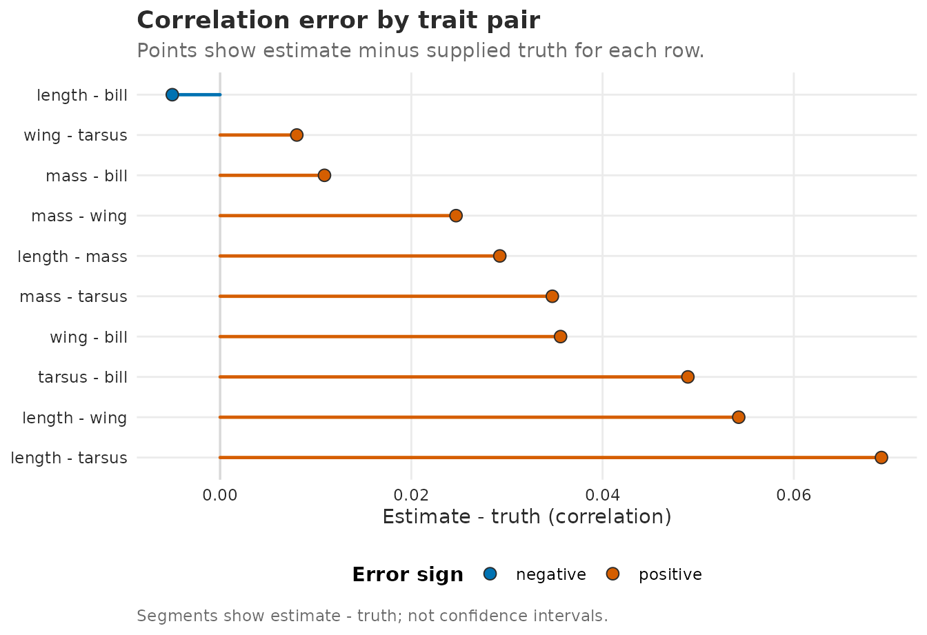

Trait-pair correlation errors from the total between-unit covariance Sigma_B = Lambda Lambda^T + Psi. Points show fitted minus true correlation; zero means exact recovery for that pair.

What extract_Sigma(level = "unit")$Sigma returns. The total between-unit covariance $\boldsymbol\Sigma_B = \boldsymbol\Lambda \boldsymbol\Lambda^{\!\top} + \boldsymbol\Psi$ — the sum of the reduced-rank shared component and the diagonal unique component. If you request latent(..., unique = FALSE), $\boldsymbol\Psi = 0$ and you get only $\boldsymbol\Lambda \boldsymbol\Lambda^{\!\top}$ , which understates the diagonal for this data-generating process. The default latent() fit above includes $\boldsymbol\Psi$ . Use part = "shared" / part = "unique" to pull just one component.

Pairwise correlations and communality

For inference on individual cross-trait correlations or per-trait communality, the canonical extractors return tidy data frames. extract_correlations() defaults to point estimates. Fisher-z bounds are an opt-in sensitivity display, not a calibrated mixed-model interval. The table below therefore reports the fitted correlations without implying universal coverage. The table is useful for reporting exact numbers; the plot shows which trait pairs have the strongest evidence of positive or negative association. Communality point estimates are enough for this first worked example. When interval estimates matter, prefer profile or Wald-style intervals where the target supports them. Bootstrap is a slower, deliberate option for a separate cached check. This article loads a small cached bootstrap_Sigma() object for the correlation figure so pkgdown does not refit bootstrap replicates while rendering.

corr_rows <- extract_correlations(fit, tier = "unit")
corr_rows
#>    tier trait_i trait_j correlation lower upper method interval_status
#> 1     B  length    mass   0.9041350    NA    NA   none            none
#> 2     B  length    wing   0.7446723    NA    NA   none            none
#> 3     B    mass    wing   0.6990173    NA    NA   none            none
#> 4     B  length  tarsus   0.7041940    NA    NA   none            none
#> 5     B    mass  tarsus   0.6407146    NA    NA   none            none
#> 6     B    wing  tarsus   0.8275512    NA    NA   none            none
#> 7     B  length    bill   0.6371630    NA    NA   none            none
#> 8     B    mass    bill   0.7217348    NA    NA   none            none
#> 9     B    wing    bill   0.2885881    NA    NA   none            none
#> 10    B  tarsus    bill   0.1853213    NA    NA   none            none

plot_correlations(morph_boot_R, tier = "unit", style = "eye", sort = "trait")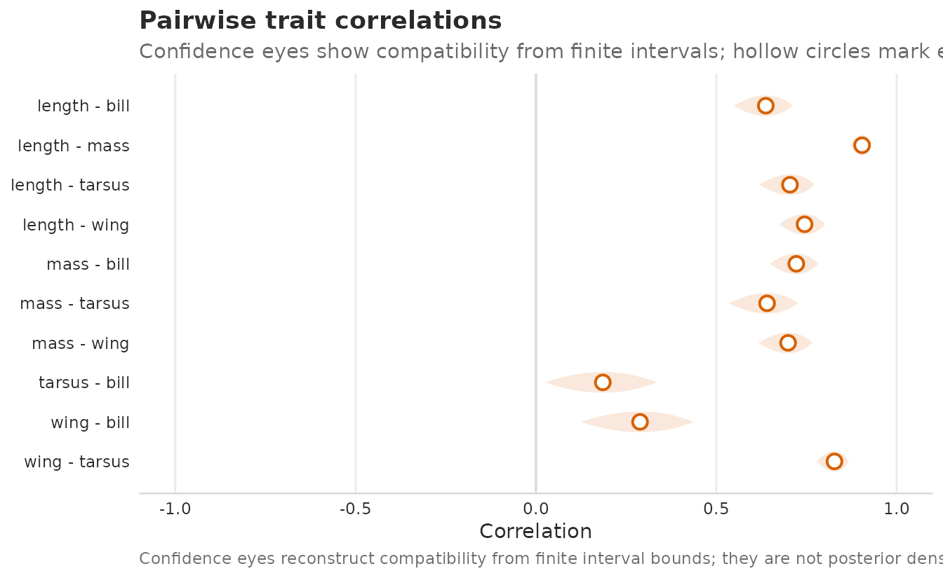

Pairwise between-individual trait correlations from a cached morphometrics bootstrap fixture. Confidence eyes reconstruct frequentist compatibility from percentile intervals; hollow circles mark estimates. Use a larger bootstrap run before making a final interval-calibration claim.

In this teaching fit, all unit-tier trait correlations are positive, so the figure mainly ranks their strength along the shared size axis. Tight confidence eyes near 1 are supplied by the cached bootstrap object (n_boot = 100, failed refits = 4). Treat this as a rendered plotting example; final inference should use a bootstrap size chosen for the study rather than the article’s lightweight fixture.

The same cached intervals can be shown as a matrix-style ellipse plot. Here the shape and fill show the sign and strength of each correlation; black borders and stars mark pairs whose supplied bootstrap interval does not cross zero. The stars are a display convention on the cached fixture’s percentile intervals, not a calibrated significance test — choose a bootstrap size for the study before drawing inferential conclusions.

plot(fit, type = "correlation_ellipse", level = "unit", boot = morph_boot_R)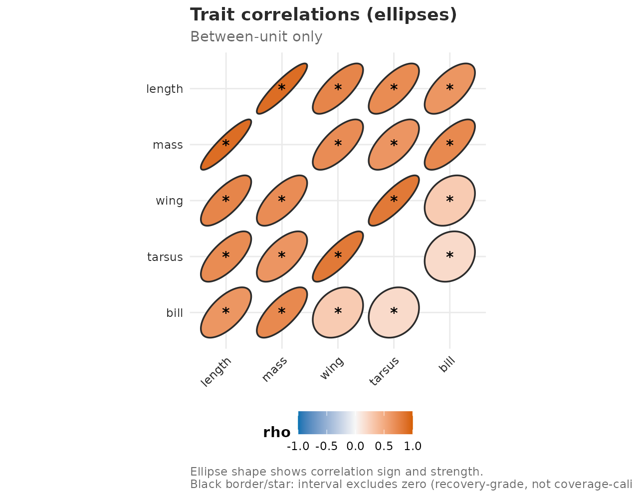

Ellipse view of the same cached between-individual correlation intervals. Ellipse tilt and colour show the fitted correlation; black borders and stars mark bootstrap percentile intervals that do not cross zero.

extract_communality(fit, level = "unit")
#>    length      mass      wing    tarsus      bill 
#> 0.8911057 0.9348032 0.8055346 0.8684255 0.7801652

Communality $c_t^2 = (\boldsymbol\Lambda\boldsymbol\Lambda^{\!\top})_{tt} / \boldsymbol\Sigma_{B,tt}$ is the fraction of trait $t$ ’s variance shared with the others via the latent factors; high $c_t^2$ means strongly integrated, low $c_t^2$ means trait-specific variation dominates.

This single generated data set is a teaching example, not a full simulation study. For this known fixture, the long and wide formulas recover the same off-diagonal covariance pattern. Broader coverage and interval-calibration claims require separate simulation studies across prespecified generating values, with every failed fit included in the accounting.

Why default `latent()`? `dep` and `indep` on the same data

The morphometric workflow uses ordinary latent(d = K) to estimate $\boldsymbol\Sigma_B = \boldsymbol\Lambda\boldsymbol\Lambda^\top + \boldsymbol{\Psi}$ . Two alternative covstruct modes — dep (full unstructured $\boldsymbol\Sigma_B$ with $T(T+1)/2$ free entries) and indep (diagonal-only $\boldsymbol\Sigma_B = \mathrm{diag}(\sigma^2_1, \dots, \sigma^2_T)$ , no cross-trait modelling) — are also valid keywords. Refit the same data under each to see what the user actually loses or gains. These are ordinary unit-tier keywords; source-specific forms such as phylo_dep() and spatial_dep() affect phylogenetic or spatial unit-tier covariance instead.

fit_full_long <- gllvmTMB(
  value ~ 0 + trait +
          latent(0 + trait | individual, d = T),
  data = df, trait = "trait", unit = "individual"
)
fit_full_wide <- gllvmTMB(
  traits(length, mass, wing, tarsus, bill) ~ 1 +
          latent(1 | individual, d = T),
  data = df_wide, unit = "individual"
)

fit_dep_long <- gllvmTMB(
  value ~ 0 + trait +
          dep(0 + trait | individual),
  data = df, trait = "trait", unit = "individual"
)
fit_dep_wide <- gllvmTMB(
  traits(length, mass, wing, tarsus, bill) ~ 1 +
          dep(1 | individual),
  data = df_wide, unit = "individual"
)

fit_indep_long <- gllvmTMB(
  value ~ 0 + trait +
          indep(0 + trait | individual),
  data = df, trait = "trait", unit = "individual"
)
fit_indep_wide <- gllvmTMB(
  traits(length, mass, wing, tarsus, bill) ~ 1 +
          indep(1 | individual),
  data = df_wide, unit = "individual"
)

fit_full  <- fit_full_long
fit_dep   <- fit_dep_long
fit_indep <- fit_indep_long

cat("Max long/wide logLik difference across comparison fits:",
    signif(max(abs(c(
      as.numeric(logLik(fit_full_long)) - as.numeric(logLik(fit_full_wide)),
      as.numeric(logLik(fit_dep_long)) - as.numeric(logLik(fit_dep_wide)),
      as.numeric(logLik(fit_indep_long)) - as.numeric(logLik(fit_indep_wide))
    ))), 3),
    "\n")
#> Max long/wide logLik difference across comparison fits: 0

S1 <- extract_Sigma(fit,       level = "unit")$Sigma
S2 <- extract_Sigma(fit_full,  level = "unit")$Sigma
S3 <- extract_Sigma(fit_dep,   level = "unit")$Sigma
S4 <- extract_Sigma(fit_indep, level = "unit")$Sigma

off       <- function(M) M[upper.tri(M)]
truth_off <- off(Sigma_true)
ll        <- function(f) round(as.numeric(logLik(f)), 2)

data.frame(
  mode               = c("latent(d=2)", "latent(d=T)",
                         "dep", "indep"),
  logL               = c(ll(fit), ll(fit_full), ll(fit_dep), ll(fit_indep)),
  off_diag_corr_truth = c(round(cor(off(S1), truth_off), 3),
                          round(cor(off(S2), truth_off), 3),
                          round(cor(off(S3), truth_off), 3),
                          NA),
  diag_min_max        = c(sprintf("%.2f - %.2f", min(diag(S1)), max(diag(S1))),
                          sprintf("%.2f - %.2f", min(diag(S2)), max(diag(S2))),
                          sprintf("%.2f - %.2f", min(diag(S3)), max(diag(S3))),
                          sprintf("%.2f - %.2f", min(diag(S4)), max(diag(S4))))
)
#>          mode     logL off_diag_corr_truth diag_min_max
#> 1 latent(d=2)  -739.61               0.989  0.93 - 1.33
#> 2 latent(d=T)  -739.45               0.989  0.93 - 1.33
#> 3         dep  -739.45               0.989  0.87 - 1.26
#> 4       indep -1103.01                  NA  0.93 - 1.33

What this shows:

dep and latent(d = T) both recover the saturated covariance surface — the comparison is a useful check that the dense fit and the full-rank latent parameterisation agree on the covariance pattern. dep and latent(d = T) give the same saturated fit here — numerically equal logL and $\boldsymbol\Sigma_B$ on this fixture.
Reduced-rank latent(d = 2) with default $\boldsymbol\Psi$ matches the saturated fit within 0.1 nats of logL. With $T = 5$ traits and a rank-2 truth, the rank constraint loses essentially no information and gives the same off-diagonal correlation pattern as the saturated fit ( $r$ vs truth ≈ 0.95 for both).
indep recovers the diagonals fine — Gaussian gives per-trait identifiability for the marginal variance even with no cross-trait modelling — but loses every off-diagonal. The off-diagonal correlation with truth is NA because the fitted off-diagonals are exactly zero by construction. logL is materially worse.

For this simulated rank-2 Gaussian truth, default latent(d = 2) and the saturated dep fit recover nearly the same covariance pattern, while indep cannot recover off-diagonal association because it sets those entries to zero by construction. Pick latent(d = K) when you have a strong rank- $K$ hypothesis (size + shape, here); fall back to dep if you suspect $K \approx T$ and want the saturated fit; reach for indep only when you genuinely believe traits are mutually independent.

What the latent factors mean

Every factor model has a rotational ambiguity: $\boldsymbol\Lambda$ and $\boldsymbol\Lambda \mathbf{Q}$ produce the same $\boldsymbol\Sigma_B$ for any orthogonal $\mathbf{Q}$ . To compare loadings between fits or between packages, rotate to a standard convention (varimax for interpretability, or lower-triangular for a unique fit):

L_hat <- extract_ordination(fit, level = "unit")$loadings
rot   <- rotate_loadings(
  fit,
  level = "unit",
  method = "varimax",
  anchor_traits = c("mass", "wing")
)
round(rot$Lambda, 2)
#>         LV1  LV2
#> length 0.72 0.73
#> mass   0.67 0.89
#> wing   0.92 0.28
#> tarsus 0.92 0.14
#> bill   0.07 0.85

The same convention is available as tidy rows when you want a table beside the figure:

loading_table <- extract_rotated_loadings_table(
  fit,
  level = "unit",
  method = "varimax",
  anchor_traits = c("mass", "wing"),
  loading_scale = "standardized"
)

loading_table <- loading_table[
  order(loading_table$axis, -loading_table$abs_loading),
  c("trait", "axis", "loading", "axis_share", "anchor_trait")
]
head(loading_table, 8)
#>     trait axis    loading axis_share anchor_trait
#> 4  tarsus  LV1 0.92167242  0.5537047         mass
#> 3    wing  LV1 0.85907137  0.5537047         mass
#> 1  length  LV1 0.66380729  0.5537047         mass
#> 2    mass  LV1 0.57959588  0.5537047         mass
#> 5    bill  LV1 0.06957319  0.5537047         mass
#> 10   bill  LV2 0.88052530  0.4462953         wing
#> 7    mass  LV2 0.77386811  0.4462953         wing
#> 6  length  LV2 0.67116734  0.4462953         wing

ord <- extract_ordination(fit, level = "unit")
head(ord$scores)
#>          LV1         LV2
#> 1 -0.4370449  1.29664647
#> 2  0.2975838  0.29257732
#> 3  2.4105980 -1.02649382
#> 4  2.0998041 -0.02503290
#> 5  1.3894629  0.10884484
#> 6 -0.4262655  0.03733953
plot(
  fit,
  type = "ordination",
  level = "unit",
  anchor_traits = c("mass", "wing"),
  standardize_loadings = TRUE
) +
  ggplot2::labs(
    caption = paste(
      "Grey points are latent scores; arrows are standardized loadings.",
      "Axes use varimax rotation with sign anchors on mass and wing.",
      "Use Sigma and correlation summaries for rotation-invariant interpretation.",
      sep = "\n"
    )
  )

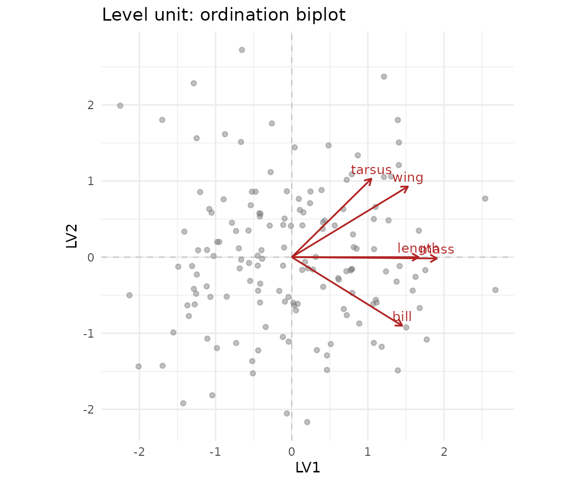
Ordination of the fitted morphometrics model. Grey points show individual latent scores; arrows show standardized trait loadings. Mass and wing anchor the displayed axis signs, but axis sign and orientation remain conventions. Individuals spread mainly along a shared body-size direction, while arrow angles show how the five traits align with the two displayed axes.

This ordination comes from the fitted covariance model ( $\boldsymbol\Sigma = \boldsymbol\Lambda\boldsymbol\Lambda^\top + \boldsymbol\Psi$ ): unlike PCA or NMDS, the axes are estimated latent quantities rather than an eigen- or distance-decomposition of the raw data. Their uncertainty is not shown in this plot, and the grey points are predicted latent scores (empirical-Bayes conditional modes of $\mathbf{u}_i$ ), not observed coordinates.

The biplot shows the trait loadings on the two latent axes. In a real morphometric study, the first axis usually picks up overall size, with all traits loading positively — the famous “general factor” of body size. The second axis picks up shape contrasts. The sign anchor is a reporting convention: here positive LV1 is anchored to mass and positive LV2 to wing; changing signs would not change the fitted covariance.

What this article does not cover

This is the simplest case on the complexity ladder. Richer models — binary / joint species distribution responses, phylogenetic and spatial dependence between rows, and two-level between/within designs — build on this same latent() foundation and are covered in their own guides as they become public.