Functional biogeography GLLVM: M1 to M2 to extensions

The replicated site–species–trait GLLVM is the canonical functional-biogeography model of Nakagawa et al. (in prep). This article fits it as a two-step model ladder:

§1 – M1 (functional integration core). Trait covariation decomposed into a between-site component $\boldsymbol{\Sigma}_B$ (global functional integration) and a within-site component $\boldsymbol{\Sigma}_W$ (local functional integration). No space, no phylogeny – just the syndrome story.
§2 – M2 (controls for space and phylogeny). Re-fit M1 with spatial and phylogenetic adjustment terms. Compare M2’s $\boldsymbol{\Sigma}_B$ / $\boldsymbol{\Sigma}_W$ to M1’s. If the syndrome story holds, the controls have done their job.
§3 – Extensions. Promote space or phylogeny to its own covariance decomposition (M3, M4) when the inferential target is spatial or phylogenetically conserved trait syndromes. We preview the syntax and point at companion articles; the fits themselves live elsewhere.

A family of models

Before §1, the conceptual scaffolding. The replicated site–species–trait GLLVM is one of a family of trait-covariance models. The right model depends on the response shape:

Data / question	Recommended model
Species occurrences/abundances; traits explain species responses	Site $\times$ species JSDM / fourth-corner GLLVM (`joint-sdm`)
One CWM/functional summary per site and trait	Site-summary / CWM site $\times$ trait GLLVM
Species-in-site trait observations, enough within-site richness	Replicated site–species–trait GLLVM (this article)
Species have one trait value each (AVONET-style)	Two-stage site-summary model (`corvidae-two-stage`)
Trait-state counts or functional-gene frequencies	Trait-state abundance/count GLLVM
Trait integration across species/evolution	Species $\times$ trait phylogenetic GLLVM (`phylogenetic-gllvm`)

This article models direct trait observations $y_{sit}$ on multiple species at each site. The other rows of the table point at the right article for the other response shapes; do not force this model onto the wrong one.

A second conceptual move runs through §1 and §2: the adjustment vs partitioning distinction for spatial and phylogenetic terms.

Adjustment models (M2, this article’s main focus). Spatial and phylogenetic terms are controls, so the primary biological targets remain $\boldsymbol{\Sigma}_B$ and $\boldsymbol{\Sigma}_W$ . Use spatial_unique() and phylo_unique() – per-trait variances on a shared correlation structure ( $\mathbf{K}_{\text{space}}$ and $\mathbf{C}_{\text{phy}}$ ).
Partitioning models (M3, M4 in §3). Spatial and phylogenetic signals get their own reduced-rank covariance decomposition ( $\boldsymbol{\Sigma}_R$ , $\boldsymbol{\Sigma}_P$ ) via spatial_latent + spatial_unique and phylo_latent + phylo_unique. The question shifts to: are syndromes spatially structured or phylogenetically conserved? These models are more data-demanding; treat them as sensitivity analyses.

Setup and DGP

library(gllvmTMB)
library(ape)
library(ggplot2)

Wide-format input. The data here are naturally long (one row per (site, species, trait) cell), but field datasets sometimes arrive wide (one row per (site, species), one column per trait). The formula-wide path keeps that shape readable: traits(trait_1, ..., trait_T) ~ 1 + latent(1 | site_species, d = 2) + unique(1 | site_species). The long form below stays canonical because it keeps site, species, and site_species visible for the crossed ecological interpretation.

A 60-site, 30-species, 6-trait fixture with mean 5 species per site (300 rows-ish) gives both M1 and M2 enough information to recover the simulation truth on the largest covariance entries. The DGP includes:

a rank-2 between-site truth ( $d_B = 2$ ): two trait syndromes with opposite signs across the two trait blocks (1-3 vs 4-6);
a rank-1 within-site truth ( $d_W = 1$ ): a single shared local axis;
small phylogenetic and spatial signals so M2 has something to control for, but small enough that the M1-vs-M2 comparison is honest – the syndrome story should not be an artefact of geography or shared ancestry.

set.seed(42)
n_sites   <- 60
n_species <- 30
n_traits  <- 6

tree <- ape::rcoal(n_species)
tree$tip.label <- paste0("sp", seq_len(n_species))

## Two clear syndromes (rank d_B = 2 truth)
Lambda_B_true <- matrix(c(
   0.9,  0.7,  0.6, -0.2, -0.5, -0.3,    # axis 1 (traits 1-3 high; 4-6 low)
   0.2, -0.1,  0.0,  0.7,  0.7,  0.5     # axis 2 (traits 4-6 high)
), nrow = n_traits, ncol = 2)
Lambda_W_true <- matrix(c(0.5, 0.4, 0.3, 0.4, 0.3, 0.2),
                        nrow = n_traits, ncol = 1)
S_B_true <- rep(0.15, n_traits)
S_W_true <- rep(0.20, n_traits)

sim <- simulate_site_trait(
  n_sites = n_sites, n_species = n_species, n_traits = n_traits,
  mean_species_per_site = 5,
  Lambda_B = Lambda_B_true, Lambda_W = Lambda_W_true,
  S_B = S_B_true, S_W = S_W_true,
  Cphy = ape::vcv(tree, corr = TRUE),
  sigma2_phy    = rep(0.10, n_traits),
  sigma2_sp     = rep(0.05, n_traits),
  spatial_range = 0.4,
  sigma2_spa    = rep(0.10, n_traits),
  sigma2_eps    = 0.10,
  seed          = 42
)
df <- sim$data
levels(df$species) <- tree$tip.label

Sigma_B_true <- Lambda_B_true %*% t(Lambda_B_true) + diag(S_B_true)
Sigma_W_true <- Lambda_W_true %*% t(Lambda_W_true) + diag(S_W_true)

§1 – M1: functional integration core

The lead-in model. No space, no phylogeny. The mean structure is

$\mu_{st} = \alpha_t + \mathbf{x}_s^{\!\top} \boldsymbol{\beta}_t,$

a per-trait intercept $\alpha_t$ plus per-trait slopes $\boldsymbol{\beta}_t$ on two site-level predictors env_1, env_2. The random-effect structure is

$y_{sit} = \mu_{st} + u_{st} + e_{sit} + \delta_{sit},$

with

$\mathbf{u}_s \sim \mathcal{N}(\mathbf{0}, \boldsymbol{\Sigma}_B)$ , $\boldsymbol{\Sigma}_B = \boldsymbol{\Lambda}_B \boldsymbol{\Lambda}_B^{\!\top} + \boldsymbol{\Psi}_B$ – global functional integration, between-site trait covariance.
$\mathbf{e}_{si} \sim \mathcal{N}(\mathbf{0}, \boldsymbol{\Sigma}_W)$ , $\boldsymbol{\Sigma}_W = \boldsymbol{\Lambda}_W \boldsymbol{\Lambda}_W^{\!\top} + \boldsymbol{\Psi}_W$ – local functional integration, within-site species deviations.
$\delta_{sit} \sim \mathcal{N}(0, \sigma^2_\delta)$ – residual.

gllvmTMB syntax:

t0 <- Sys.time()
fit_M1 <- gllvmTMB(
  value ~ 0 + trait +
          (0 + trait):env_1 + (0 + trait):env_2 +
          latent(0 + trait | site, d = 2) +
          unique(0 + trait | site) +
          latent(0 + trait | site_species, d = 1) +
          unique(0 + trait | site_species),
  data    = df,
  cluster = "species"
)
t_M1 <- round(as.numeric(Sys.time() - t0, units = "secs"), 1)
fit_M1$opt$convergence
#> [1] 0

Wall time: 2.9 s. Extract $\boldsymbol{\Sigma}_B$ and $\boldsymbol{\Sigma}_W$ :

Sigma_B_M1 <- extract_Sigma(fit_M1, level = "unit",     part = "total")$Sigma
Sigma_W_M1 <- extract_Sigma(fit_M1, level = "unit_obs", part = "total")$Sigma
round(Sigma_B_M1, 2)
#>         trait_1 trait_2 trait_3 trait_4 trait_5 trait_6
#> trait_1    1.01    0.68    0.57   -0.21   -0.47   -0.15
#> trait_2    0.68    0.82    0.47   -0.30   -0.52   -0.24
#> trait_3    0.57    0.47    0.57   -0.28   -0.46   -0.22
#> trait_4   -0.21   -0.30   -0.28    0.65    0.53    0.34
#> trait_5   -0.47   -0.52   -0.46    0.53    0.99    0.44
#> trait_6   -0.15   -0.24   -0.22    0.34    0.44    0.59
round(Sigma_W_M1, 2)
#>         trait_1 trait_2 trait_3 trait_4 trait_5 trait_6
#> trait_1    0.73    0.22    0.15    0.21    0.17    0.15
#> trait_2    0.22    0.58    0.13    0.18    0.15    0.13
#> trait_3    0.15    0.13    0.44    0.13    0.11    0.09
#> trait_4    0.21    0.18    0.13    0.62    0.14    0.12
#> trait_5    0.17    0.15    0.11    0.14    0.47    0.10
#> trait_6    0.15    0.13    0.09    0.12    0.10    0.48

The block structure is recovered: traits 1-3 covary positively, traits 4-6 covary positively, and the two blocks covary negatively – matching the rank-2 simulation truth. Per-trait communality $c^2_{B,t} = (\boldsymbol{\Lambda}_B \boldsymbol{\Lambda}_B^{\!\top})_{tt} / (\boldsymbol{\Sigma}_B)_{tt}$ and the site-level ICC $R^{(\text{site})}_t = (\boldsymbol{\Sigma}_B)_{tt} / [(\boldsymbol{\Sigma}_B)_{tt} + (\boldsymbol{\Sigma}_W)_{tt}]$ :

round(extract_communality(fit_M1, level = "unit"), 3)
#> trait_1 trait_2 trait_3 trait_4 trait_5 trait_6 
#>   0.948   0.672   0.712   0.626   0.756   0.493
round(extract_ICC_site(fit_M1), 3)
#> trait_1 trait_2 trait_3 trait_4 trait_5 trait_6 
#>   0.582   0.583   0.566   0.512   0.677   0.549

Three things to watch for in any M1 fit, each a separate identifiability concern:

Note (1) – $\boldsymbol{\Sigma}_W$ vs $\sigma_\delta$ identifiability. With no within-cell replication (one observation per (site, species, trait) triple), only the sum $\boldsymbol{\Sigma}_W^{*} = \boldsymbol{\Sigma}_W + \mathrm{diag}(\sigma^2_\delta)$ is identified. The engine handles this by auto-suppressing sigma_eps to a tiny floor whenever a per-row unique() is present (you’ll see a one-shot inform when M1 fits). Replication within cell – multiple individuals of the same species at the same site, or repeated visits – is the design move that splits them. See pitfalls for a worked demonstration.

Note (2) – communality is rank-conditional. $c^2_{B,t}$ depends on the choice of $d_B$ . Refitting M1 at $d_B = 1$ on the same data gives different communalities than at $d_B = 2$ :

fit_M1_d1 <- gllvmTMB(
  value ~ 0 + trait +
          (0 + trait):env_1 + (0 + trait):env_2 +
          latent(0 + trait | site, d = 1) +
          unique(0 + trait | site) +
          latent(0 + trait | site_species, d = 1) +
          unique(0 + trait | site_species),
  data    = df,
  cluster = "species"
)
rbind(
  d_B_1 = round(extract_communality(fit_M1_d1, level = "unit"), 3),
  d_B_2 = round(extract_communality(fit_M1,    level = "unit"), 3)
)
#>       trait_1 trait_2 trait_3 trait_4 trait_5 trait_6
#> d_B_1   0.628   0.677   0.727   0.417   0.665   0.304
#> d_B_2   0.948   0.672   0.712   0.626   0.756   0.493

The two communality vectors disagree by 0.05–0.4 across traits. The reason is structural: $c^2_{B,t}$ is the diagonal of $\boldsymbol{\Lambda}_B \boldsymbol{\Lambda}_B^{\!\top}$ over the diagonal of $\boldsymbol{\Sigma}_B$ , and shrinking $d_B$ by one takes a column out of $\boldsymbol{\Lambda}_B$ . Always report the rank you used. Pick $d_B$ on a model-comparison criterion (AIC, cross-validated likelihood) before reporting communality, not after.

Note (3) – the response shape determines the question. This article uses direct trait observations $y_{sit}$ . For occurrence/abundance data with traits as covariates, fit a JSDM / fourth-corner GLLVM (joint-sdm). For one CWM-style summary per site, use the site-summary CWM model. For AVONET-style data with one trait value per species, use the two-stage workflow. The replicated site–species–trait model below is right for our DGP; do not force it onto a different one.

§2 – M2: spatial and phylogenetic adjustment

Same equation as §1 but with four extra random-effect terms:

$y_{sit} = \mu_{st} + u_{st} + e_{sit} + r_{st} + p_{it} + q_{it} + \delta_{sit},$

with

$r_{\cdot t} \sim \mathcal{N}(\mathbf{0}, \sigma^2_{R,t}\,\mathbf{K}_{\text{space}})$ – per-trait Matérn spatial field on the SPDE mesh; spatial control.
$p_{\cdot t} \sim \mathcal{N}(\mathbf{0}, \sigma^2_{P,t}\,\mathbf{C}_{\text{phy}})$ – per-trait phylogenetic species random effect on the shared $\mathbf{C}_{\text{phy}}$ ; phylogenetic control.
$q_{\cdot t} \sim \mathcal{N}(\mathbf{0}, \sigma^2_{Q,t}\,\mathbf{I})$ – per-trait non-phylogenetic species random effect (independent across species); the residual species effect after phylogeny.

These are the adjustment-mode terms: each trait carries its own variance on a shared correlation structure ( $\mathbf{K}_{\text{space}}$ , $\mathbf{C}_{\text{phy}}$ , $\mathbf{I}$ ), without introducing a cross-trait spatial or phylogenetic loading matrix. This keeps the focal interpretation on $\boldsymbol{\Sigma}_B$ and $\boldsymbol{\Sigma}_W$ .

The $p_{it} + q_{it}$ pair is the same Hadfield–Nakagawa (2010) decomposition used in the phylogenetic-gllvm article, just placed at the cluster (species) slot of a crossed (site $\times$ species) fit rather than at the unit slot of a per-species fit. The two correlation matrices $\mathbf{C}_{\text{phy}}$ and $\mathbf{I}$ are orthogonal, so $\sigma^2_{P,t}$ and $\sigma^2_{Q,t}$ are jointly identifiable – see the note after the fit for the empirical regime.

mesh <- make_mesh(df, c("lon", "lat"), cutoff = 0.1)

t0 <- Sys.time()
fit_M2 <- gllvmTMB(
  value ~ 0 + trait +
          (0 + trait):env_1 + (0 + trait):env_2 +
          spatial_unique(0 + trait | coords, mesh = mesh) +
          latent(0 + trait | site, d = 2) +
          unique(0 + trait | site) +
          latent(0 + trait | site_species, d = 1) +
          unique(0 + trait | site_species) +
          unique(0 + trait | species) +              # q_it
          phylo_unique(species, tree = tree),         # p_it
  data    = df,
  cluster = "species"
)
t_M2 <- round(as.numeric(Sys.time() - t0, units = "secs"), 1)
fit_M2$opt$convergence
#> [1] 0

Wall time: 18.2 s.

A note on identifiability. With $n_{\text{species}} \geq 100$ and a crossed (site $\times$ species) design, $\sigma^2_{Q,t}$ recovers within $$10% relative error and $\sigma^2_{P,t}$ within $$50% (per-trait estimates can be noisy when one trait’s phylogenetic signal is weak; the trait-averaged $\bar{\sigma}^2_P$ is more stable). At small $n_{\text{species}}$ or weak phylogenetic signal, the $p_{it}$ and $q_{it}$ pieces cannot be cleanly separated and one should compare M1 (without unique(0 + trait | species)) to M2 (with it) to confirm both terms contribute on the focal data. The engine prints a one-shot informational note pointing at this regime when it detects the pairing.

The pedagogical moment: do the controls move the syndrome?

Re-extract $\boldsymbol{\Sigma}_B$ and $\boldsymbol{\Sigma}_W$ from M2 and compare to M1’s:

Sigma_B_M2 <- extract_Sigma(fit_M2, level = "unit",     part = "total")$Sigma
Sigma_W_M2 <- extract_Sigma(fit_M2, level = "unit_obs", part = "total")$Sigma

R_B_M1 <- extract_Sigma(fit_M1, level = "unit")$R
R_B_M2 <- extract_Sigma(fit_M2, level = "unit")$R
R_W_M1 <- extract_Sigma(fit_M1, level = "unit_obs")$R
R_W_M2 <- extract_Sigma(fit_M2, level = "unit_obs")$R

c(max_abs_diff_R_B = round(max(abs(R_B_M2 - R_B_M1)), 3),
  max_abs_diff_R_W = round(max(abs(R_W_M2 - R_W_M1)), 3))
#> max_abs_diff_R_B max_abs_diff_R_W 
#>            0.157            0.166

Side-by-side correlation-matrix heatmaps:

heatmap_df <- function(R, label) {
  rn <- rownames(R) %||% paste0("trait_", seq_len(nrow(R)))
  data.frame(
    model  = label,
    trait_i = factor(rep(rn, ncol(R)), levels = rn),
    trait_j = factor(rep(rn, each = nrow(R)), levels = rn),
    rho     = as.vector(R)
  )
}

R_B_long <- rbind(
  heatmap_df(R_B_M1, "M1 (no controls)"),
  heatmap_df(R_B_M2, "M2 (+ space + phylo)")
)

ggplot(R_B_long, aes(trait_i, trait_j, fill = rho)) +
  geom_tile(colour = "white") +
  geom_text(aes(label = sprintf("%.2f", rho)), size = 2.8) +
  scale_fill_gradient2(low = "#1f78b4", mid = "white", high = "#b2182b",
                       midpoint = 0, limits = c(-1, 1)) +
  facet_wrap(~ model) +
  coord_equal() +
  labs(x = NULL, y = NULL,
       title = expression("Between-site trait correlations " *
                          R[B] * " = cor(" * Sigma[B] * ")")) +
  theme_minimal(base_size = 11) +
  theme(panel.grid = element_blank(),
        axis.text.x = element_text(angle = 45, hjust = 1))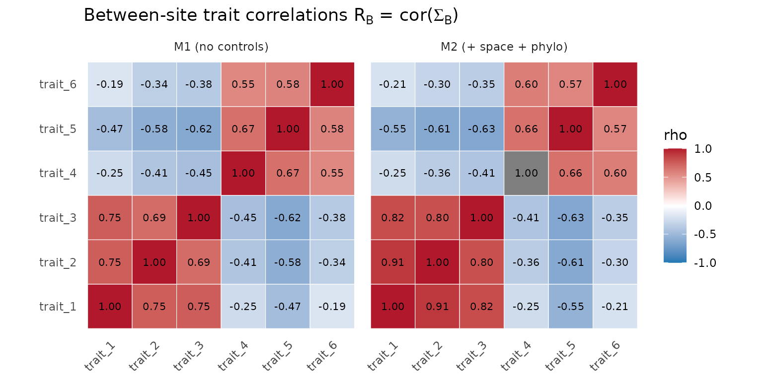

Cross-trait correlation matrix at the between-site (Sigma_B) tier under M1 (no controls) and M2 (spatial + phylogenetic adjustment). The block structure (traits 1-3 vs 4-6) is preserved across models.

R_W_long <- rbind(
  heatmap_df(R_W_M1, "M1 (no controls)"),
  heatmap_df(R_W_M2, "M2 (+ space + phylo)")
)

ggplot(R_W_long, aes(trait_i, trait_j, fill = rho)) +
  geom_tile(colour = "white") +
  geom_text(aes(label = sprintf("%.2f", rho)), size = 2.8) +
  scale_fill_gradient2(low = "#1f78b4", mid = "white", high = "#b2182b",
                       midpoint = 0, limits = c(-1, 1)) +
  facet_wrap(~ model) +
  coord_equal() +
  labs(x = NULL, y = NULL,
       title = expression("Within-site trait correlations " *
                          R[W] * " = cor(" * Sigma[W] * ")")) +
  theme_minimal(base_size = 11) +
  theme(panel.grid = element_blank(),
        axis.text.x = element_text(angle = 45, hjust = 1))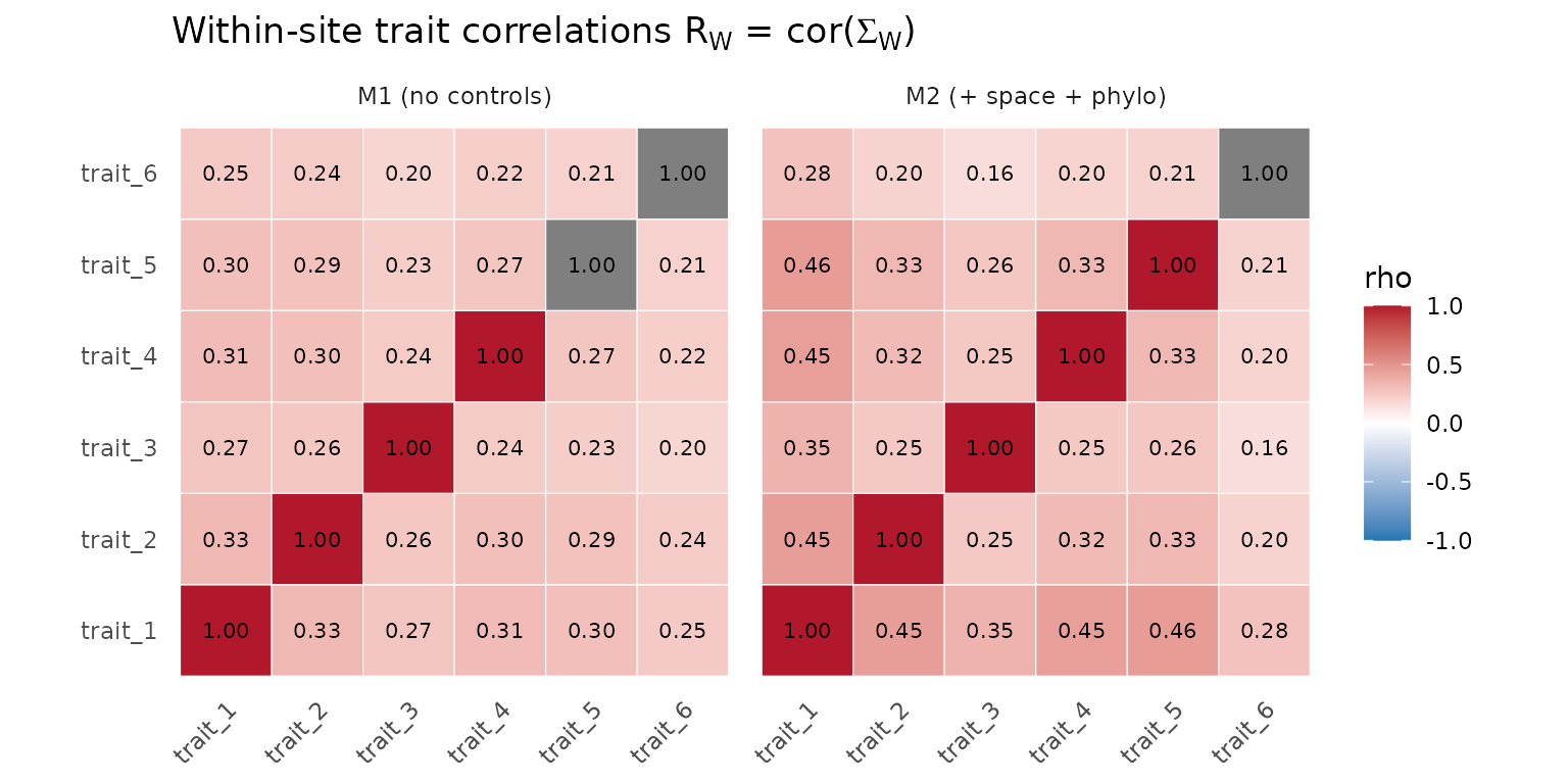

Cross-trait correlation matrix at the within-site (Sigma_W) tier under M1 and M2. The local-integration story is similarly stable to the addition of controls.

The block structure of $\mathbf{R}_B$ – traits 1-3 positively correlated, traits 4-6 positively correlated, the two blocks negatively correlated – is the same under M1 and M2. That is the desired finding. It tells the reader the syndrome was not a geography or ancestry artefact: even after controlling for the spatial and phylogenetic structure that the data carry, the same two syndromes survive.

If the comparison instead showed M2’s $\mathbf{R}_B$ flattening (syndrome erased) or shifting sign (syndrome reversed), you would have a different and equally interesting story: the apparent global functional integration was largely a function of spatial covariation in the environmental drivers, or of shared ancestry. Either finding should be reported – the M1 vs M2 comparison is the diagnostic for which.

Sample size guidance. M2 is a multi-tier model with five random-effect tiers and ~70 free parameters at $T = 6$ . Identifiability requires enough groups at each tier, not just enough total observations:

$n_{\text{sites}} \geq 50$ for stable $\boldsymbol{\Sigma}_B$

mean species per site $\geq 5$ for identifiable $\boldsymbol{\Sigma}_W$ (with single observation per (site, species, trait) cell, only $\boldsymbol{\Sigma}_W^{\star} = \boldsymbol{\Sigma}_W + \mathrm{diag}(\sigma^2_\delta)$ is identifiable – see Note 1 in §1)

$n_{\text{species}} \geq 50$ for the per-trait phylogenetic ( $\sigma^2_{P,t}$ ) and non-phylogenetic species ( $\sigma^2_{Q,t}$ ) variances

phylogenetic signal at moderate-or-stronger ( $\lambda_{\text{Pagel}} \gtrsim 0.4$ ) for the phylogenetic decomposition to bite

Below these thresholds, fall back to M1 – drop the controls, report $\boldsymbol{\Sigma}_B$ and $\boldsymbol{\Sigma}_W$ as partial (not “fully adjusted”) global and local integration. Don’t add tiers your data can’t support: gllvmTMB makes complex models expressible, but expressibility is not identifiability. A formal regime map across M1–M4 is in preparation (dev/design/11-identifiability-regime-map.md); a dedicated article will follow once the simulation grid completes.

§3 – Extensions: when space and phylogeny become the target

When the question is about space or phylogeny itself – “are syndromes spatially structured?”, “is one of the syndromes phylogenetically conserved?” – promote the corresponding signal from a per-trait control to a full reduced-rank covariance decomposition. We sketch the syntax for two extension models below and point at the dedicated articles for the worked fits.

M3 – spatial trait syndromes

Add a spatial_latent term in addition to spatial_unique to estimate $\boldsymbol{\Sigma}_R = \boldsymbol{\Lambda}_R\boldsymbol{\Lambda}_R^{\!\top} + \boldsymbol{\Psi}_R$ , the spatial trait-covariance decomposition. Loadings on $\boldsymbol{\Lambda}_R$ tell you which traits hang together spatially.

fit_M3 <- gllvmTMB(
  value ~ 0 + trait + (0 + trait):env_1 + (0 + trait):env_2 +
          spatial_latent(0 + trait | coords, d = 2, mesh = mesh) +
          spatial_unique(0 + trait | coords, mesh = mesh) +
          latent(0 + trait | site, d = 2) +
          unique(0 + trait | site) +
          latent(0 + trait | site_species, d = 1) +
          unique(0 + trait | site_species) +
          phylo_unique(species, tree = tree),
  data = df, cluster = "species"
)

The spatial term is the same engine as the phylogenetic two-piece decomposition documented in phylogenetic-gllvm. M3 needs more spatial signal than M2 to identify both $\boldsymbol{\Lambda}_R$ and $\boldsymbol{\Psi}_R$ separately; treat its loadings as a sensitivity analysis to M2’s per-trait spatial variances. A worked example will appear in the planned spatial-trait-syndromes article.

M4 – phylogenetically conserved syndromes

Symmetric to M3, but on the phylogeny side: pair phylo_latent with phylo_unique to estimate $\boldsymbol{\Sigma}_P = \boldsymbol{\Lambda}_P\boldsymbol{\Lambda}_P^{\!\top} + \boldsymbol{\Psi}_P$ , the phylogenetic two-piece decomposition. Loadings on $\boldsymbol{\Lambda}_P$ tell you which traits cluster together along the tree.

fit_M4 <- gllvmTMB(
  value ~ 0 + trait + (0 + trait):env_1 + (0 + trait):env_2 +
          spatial_unique(0 + trait | coords, mesh = mesh) +
          latent(0 + trait | site, d = 2) +
          unique(0 + trait | site) +
          latent(0 + trait | site_species, d = 1) +
          unique(0 + trait | site_species) +
          phylo_latent(species, d = 2, tree = tree) +
          phylo_unique(species, tree = tree),
  data = df, cluster = "species", unit = "species"  # PGLLVM mode
)

The two-piece phylogenetic fit is the focus of the phylogenetic-gllvm article and its diagnostic counterpart two-U-phylogeny. That article also covers the identifiability conditions: $K_P$ ( $d$ in phylo_latent) is identifiable up to rotation, and the two-piece split between $\boldsymbol{\Lambda}_P\boldsymbol{\Lambda}_P^{\!\top}$ and $\boldsymbol{\Psi}_P$ requires either $K_P < T$ or a constraint matrix.

What we did not fit

We deliberately do not promote the ladder beyond M4 in this article. The “kitchen-sink” model that combines latent partitioning on every tier ( $\boldsymbol{\Lambda}_B$ , $\boldsymbol{\Lambda}_W$ , $\boldsymbol{\Lambda}_R$ , $\boldsymbol{\Lambda}_P$ ) is conceptually beautiful but statistically fragile – the partitioning at one tier trades off against the others, and the loadings stop being separately identifiable without strong constraints. M2 is the sweet spot for publication-grade fits; M3 and M4 are sensitivity analyses; beyond that, the data have to carry the burden of identifiability that the model can no longer.

Diagnostics

sanity_multi(fit_M2)
#> Optimiser convergence (== 0):                PASS
#> Max |gradient| < 1.0e-02:                    PASS (max |gr| = 0.00332)
#> Hessian positive-definite:                   PASS
#> Max fixed-effect SE < 100:                   WARN (max SE = 2.58e+04)
#> latent(site, d=B) diag loadings non-zero:    PASS (min |Lambda_B diag| = 0.135)
#> latent(site_species, d=W) diag loadings non-zero: PASS (min |Lambda_W diag| = 0.61)

Convergence, max gradient, Hessian PD-ness, fixed-effect SE, and near-zero loading diagonals – the report flags any rank that was set higher than the data support. The fixed-effect SE check is the loosest filter: in fits with a phylogenetic random effect the SE column also picks up some derived sd-report quantities and can flag WARN even when the underlying fixed-effect estimates are well- behaved (compare to the tidy(fit_M2, "fixed") output). The other four checks are the ones to act on.