How to choose your model: a decision tree

gllvmTMB covers a large model space — one or two observational levels, optional phylogenetic structure, optional spatial structure, Gaussian / binary / Poisson / mixed responses, reduced-rank or full-rank trait covariance. That generality is helpful when your data are unusual but unhelpful when you are picking a formula on day 1.

This article is the decision tree we wish we had: five questions about your data, each answered with a small piece of the formula, that you assemble at the end into the model that matches your problem. If you already know the rung you want, jump to the linked article for that rung.

How to use this article

Walk down the five questions in order. At each step you pick one option, which gives you a piece of the formula or the call. By the end of section 5 you have all the pieces; section 6 shows the canonical assembled formulas for the most common combinations.

The five questions:

What does each row represent?
What is the response distribution?
Are rows phylogenetically related?
Are rows spatially organised?
Do you want a reduced-rank story for trait covariance?

The complexity ladder, at a glance

Each rung adds one structural piece to the previous. Pick the highest rung you actually need — extra structure costs identifiability and fit time. The recovery study (articles/simulation-recovery.html) quantifies how cleanly each rung’s parameters are recovered at modest n.

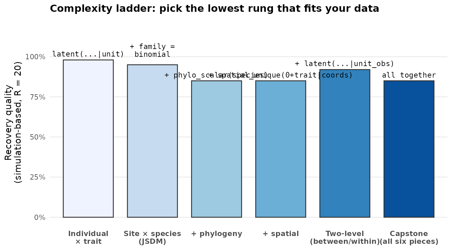
The complexity ladder: each rung adds one structural piece. Bar height = number of identifiable parameter classes recovered cleanly in the simulation-recovery study (Σ_B / Σ_W / sigma2_spa / range / lam_phy). Rungs are stacked left-to-right by complexity; pick the lowest rung that matches your data.

1. What does each row represent?

gllvmTMB is long-format: every fit takes a data frame in which each row is one (unit, trait) observation, with a value column for the response and a trait column naming which trait it is. The first decision is whether your data have one observational level or two.

Your data look like…	Observational levels	Random-effect grouping	Example article
One row per individual / site, with several traits as columns; you reshape to long format.	One: `unit`	`latent(0 + trait \| unit)`	Morphometrics (individuals × continuous traits)
Sites that each contain multiple species, with traits measured for each (site, species) combination; or repeated measures per individual; or papers with multiple items each.	Two: `site` (between) and `site_species` (within)	`latent(0 + trait \| site)` and `latent(0 + trait \| site_species)`	Corvidae two-stage and Functional biogeography

If you have a single observational level, the unit column can be called anything (individual, site, study, paper); pass its name to gllvmTMB(..., unit = "your_column"). The two-level case needs both site and site_species columns; the simulate_site_trait() helper shows the canonical layout.

2. What is the response distribution?

Latent structure is shared across response distributions, but the likelihood term per row is family-specific. Pick the family that matches your trait scale.

Trait values look like…	`family` argument	Notes
Continuous, real-valued (mass, length, log-abundance)	`family = gaussian()`	Identity link. Default.
0/1 presence-absence, yes-no, item-passed	`family = binomial()`	Logit link. Used for joint species distribution models and binary-item systematic mapping; see Joint SDM.
Counts (offspring, observations)	`family = poisson()`	Log link.
Different traits use different families	`family = list(gaussian(), binomial(), poisson())` plus a `family_var` column	One family per row. See Response families.

For the mixed-response case the family list and the family_var attribute look like this:

fam <- list(gaussian(), binomial(), poisson())
attr(fam, "family_var") <- "family"   # column on `data` selecting the row's family

If you are unsure, start with the family that matches your most abundant trait type and read the response-family reference before committing to a list.

A phylogenetic random effect is appropriate when species (or other taxa) appear repeatedly in your data and closely related taxa are likely to share trait values for evolutionary reasons. The appropriate term depends on the answer to two follow-up questions: do you want a single shared phylogenetic variance per trait, or trait-specific reduced-rank phylogenetic loadings? And how many species do you have?

Your situation	Add to formula (in-keyword `tree =` or `vcv =`)
Rows are not phylogenetically structured (e.g. individuals from one species, or sites without taxonomic identity).	Nothing.
Phylogenetic structure with one shared phylogenetic variance per trait.	`+ phylo_scalar(species, vcv = Cphy)`
Phylogenetic structure with reduced-rank trait-specific loadings (a phylogenetic version of `latent()`).	`+ phylo_latent(species, d = K, vcv = Cphy)` or `+ phylo_latent(species, d = K, tree = tree)`
Many species (n > ~200) and you want speed.	(same `phylo_latent` term) with `tree = tree` (sparse $A^{-1}$ trick); much faster than `vcv = Cphy` at this scale.

The crossover where the sparse $A^{-1}$ path overtakes the dense path sits around n_species ≈ 150-200. Above that, the speedup is roughly an order of magnitude. See Phylogenetic GLLVM for the benchmark and the choice between phylo_scalar() and phylo_latent().

4. Are rows spatially organised?

If your sites carry coordinates and you suspect residual spatial autocorrelation, add a sparse SPDE/GMRF random field. Each trait gets its own field by default.

Your situation	Add to formula	Argument to `gllvmTMB()`
Sites have no spatial structure (or you do not have coordinates).	Nothing.	—
Sites have coordinates and each trait should have its own spatial pattern.	`+ spatial_unique(0 + trait \| coords)`	`mesh = make_mesh(df, c("lon", "lat"), cutoff = ...)`
Sites have coordinates and you want one shared spatial-variance scale across traits (parsimony).	`+ spatial_scalar(0 + trait \| coords)`	`mesh = make_mesh(df, c("lon", "lat"), cutoff = ...)`
You want traits to share a low-rank spatial structure.	`+ spatial_latent(0 + trait \| coords, d = K)` — K shared SPDE fields driven by a T × K loading matrix Λ_spa.	`mesh = make_mesh(df, c("lon", "lat"), cutoff = ...)` (the spatial analogue of `phylo_latent()`).

The SPDE engine wins on speed when the dataset has more than roughly 100 sites; below that, the dense glmmTMB::exp() covariance is competitive. See SPDE benchmark for the crossover plot.

5. Do you have a reduced-rank story for trait covariance?

Even with no phylogenetic or spatial structure, you have to decide how the trait covariance itself is parameterised. This is the choice between factor analysis (a few latent dimensions explaining most cross-trait covariance) and unstructured covariance (every pair gets its own parameter).

Your situation	Add to formula	Notes
You expect a small number of latent dimensions (size, shape, life-history pace) to explain most of the cross-trait covariance. T traits, K << T factors.	`+ latent(0 + trait \| site, d = K)`	The default GLLVM choice. K = 1–3 is typical.
You want full unstructured between-unit covariance with no rank reduction.	`+ unique(0 + trait \| site)` (specific variance) plus a separate term for off-diagonal structure as needed	Reasonable when T is small (T ≤ 5) and you have many units.
Confirmatory: you know which traits load on which factor and want to pin those entries of $\boldsymbol\Lambda$ .	`+ latent(0 + trait \| site, d = K)` plus `lambda_constraint = list(B = M)`	M is a `T × K` matrix with `NA` for free entries and numeric values for fixed ones. See Lambda constraint; `?suggest_lambda_constraint` proposes a sensible matrix from a fitted unconstrained model.

For two-level models you typically include both latent() and unique() at each level, so the full between-unit piece is latent(0 + trait | site, d = K) + unique(0 + trait | site) and the within-unit piece substitutes the within-unit grouping column (e.g. site_species for site × species data, or the value passed via unit_obs = "..." for other domains). The latent() term gives the shared latent factors; the unique() term gives each trait its own residual variance on top.

6. Final formula assembly

Below are the canonical formulas for the most common combinations. The chunks below run live to confirm the formulas parse; each fits in a few seconds on the small simulations.

library(gllvmTMB)
library(ape)

6a. Individuals × continuous traits, no extra structure

The simplest case (rung 0): one level, Gaussian, no phylogeny, no space. See Morphometrics for the full walkthrough.

set.seed(1)
n_ind <- 30; n_traits <- 4
df_ind <- data.frame(
  individual = factor(rep(seq_len(n_ind), each = n_traits)),
  trait      = factor(rep(paste0("trait_", seq_len(n_traits)), n_ind),
                      levels = paste0("trait_", seq_len(n_traits))),
  value      = rnorm(n_ind * n_traits)
)
fit_ind <- gllvmTMB(
  value ~ 0 + trait + latent(0 + trait | individual, d = 2),
  data = df_ind,
  unit = "individual"
)

6b. Sites × species, presence/absence

Rung 1 with a binomial response: a joint species distribution model. See Joint SDM.

set.seed(2)
sim_b <- simulate_site_trait(
  n_sites = 30, n_species = 6, n_traits = 4,
  mean_species_per_site = 4,
  Lambda_B = matrix(rnorm(8, sd = 0.6), 4, 2),
  S_B      = rep(0.3, 4), seed = 2
)
df_b <- sim_b$data
df_b$value <- as.integer(df_b$value > 0)

fit_jsdm <- gllvmTMB(
  value ~ 0 + trait +
          latent(0 + trait | site, d = 2) +
          unique(0 + trait | site),
  data   = df_b,
  family = binomial()
)

6c. Add phylogeny

Rung 2: keep your favourite formula and add phylo_scalar() (single shared phylo variance) or phylo_latent() (reduced-rank). With a tree in hand, prefer tree = tree (in-keyword) for the sparse $A^{-1}$ path. See Phylogenetic GLLVM.

set.seed(3)
n_sp <- 8
tree <- ape::rcoal(n_sp); tree$tip.label <- paste0("sp", seq_len(n_sp))
Cphy <- ape::vcv(tree, corr = TRUE)

sim_p <- simulate_site_trait(
  n_sites = 30, n_species = n_sp, n_traits = 4,
  mean_species_per_site = 5,
  Lambda_B = matrix(rnorm(8, sd = 0.5), 4, 2),
  S_B = rep(0.3, 4),
  Cphy = Cphy, sigma2_phy = rep(0.4, 4),
  seed = 3
)
df_p <- sim_p$data
levels(df_p$species) <- tree$tip.label

fit_phy <- gllvmTMB(
  value ~ 0 + trait +
          latent(0 + trait | site, d = 2) + unique(0 + trait | site) +
          phylo_scalar(species, vcv = Cphy),
  data = df_p
)

6d. Add space

Rung 3: append spatial_unique(0 + trait | coords) and pass a mesh. The simulator places sites in [0,1]^2 automatically when spatial_range is supplied. See SPDE benchmark.

set.seed(4)
sim_s <- simulate_site_trait(
  n_sites = 40, n_species = 1, n_traits = 3,
  mean_species_per_site = 1,
  Lambda_B = matrix(0.0, 3, 1), S_B = rep(0.1, 3),
  spatial_range = 0.3, sigma2_spa = rep(0.4, 3),
  seed = 4
)
df_s <- sim_s$data
mesh <- make_mesh(df_s, c("lon", "lat"), cutoff = 0.1)

fit_spa <- gllvmTMB(
  value ~ 0 + trait + spatial_unique(0 + trait | coords, mesh = mesh),
  data = df_s
)

6e. Two-level + phylo + space (capstone)

The full Nakagawa et al. functional-biogeography model: two levels, phylogeny, and space all at once. The formula reads as a sum of the pieces from sections 1–5. The runnable end-to-end version lives in Functional biogeography; in this article we just show the formula:

fit_full <- gllvmTMB(
  value ~ 0 + trait + (0 + trait):env_1 + (0 + trait):env_2 +
          spatial_unique(0 + trait | coords, mesh = mesh) +
          latent(0 + trait | site, d = 2) +
          unique(0 + trait | site) +
          latent(0 + trait | site_species, d = 1) +
          unique(0 + trait | site_species) +
          phylo_scalar(species, vcv = Cphy),
  data = df
)

7. Diagnostic checklist

After any fit, run through these in order:

Check	How
Optimiser convergence and Hessian PD-ness.	`sanity_multi(fit)`
Implied between-unit trait covariance.	`extract_Sigma(fit, level = "unit")` (and `extract_Sigma(fit, level = "unit_obs")` for two-level fits).
Interpretable loadings.	`getLoadings(fit, level = "unit", rotate = "varimax")`
Did you fit unconstrained `latent()` with `d > 1`? Loadings are not unique.	Use `rotate = "varimax"` for a quick post-hoc rotation, or call `suggest_lambda_constraint()` to propose a confirmatory `lambda_constraint` matrix and refit.
Communalities / ICCs (manuscript Eqs. 13–15).	`extract_ICC_site(fit)`, `extract_communality(fit, level = "unit")`, `extract_communality(fit, level = "unit_obs")`

If sanity_multi() flags a non-PD Hessian or a near-zero loading diagonal, the most common causes are an over-rich model (d too large, too many latent() terms relative to data) or factor-level ordering issues in the long-format data. The Morphometrics article has a worked example of the factor-level pitfall.