gllvmTMB fits multivariate models for data where each
site, individual, species, or study has several responses. The first
question is usually not mathematical:
Which responses vary together, and how much variation is shared rather than response-specific?
This page does one small, reproducible example. It loads a prepared morphometrics object, fits the model from a wide trait table first, checks the equivalent long-data call, and extracts the covariance, correlation, communality, and ordination summaries a reader normally wants first.
gllvmTMB has an experimental lifecycle: the formula
grammar, defaults, and reported summaries and intervals may still change
as the API matures.
The fitted Gaussian model starts with observations, not with the covariance matrix. For each individual and trait, the teaching model is:
Here is the observed value for individual and trait . The intercept is the average for trait . The vector is the individual’s latent score: where that individual sits on the unobserved trait axes. The row vector says how strongly trait responds to those axes. The leftover term is the part of trait not shared with the other traits.
In generalized models, is the linear predictor and the link function connects it to the mean response: . This first example uses a Gaussian family with the identity link, so the linear predictor is the mean itself.
The R formula for that model is compact:
fit <- gllvmTMB(
  traits(length, mass, wing, tarsus, bill) ~ 1 +
    latent(1 | individual, d = 2),
  data = df_wide,
  unit = "individual",
  family = gaussian()
)
After fitting, the covariance among traits is the first report-ready summary implied by the latent part of the model:
In words: total trait covariance = shared multivariate structure +
response-specific variation. Lambda collects the trait
loadings: one row per trait and one column per latent variable. The
product Lambda Lambda^T is the shared covariance created by
those axes. Psi is the diagonal matrix of trait-specific
variance left over after the shared axes. Ordinary latent()
estimates both pieces by default.
For a first fit, read Sigma, correlations, and
communality before reading individual Lambda entries. The
latent variables can be flipped or turned without changing the
covariance they imply, so raw loading columns need a rotation or
confirmatory constraint before they become a biological story.
First fit: wide individual-by-trait morphology
We have n individuals, each measured on T
morphological traits across a few sessions. The biological question: do
the traits covary on a small number of latent variables (e.g. a
body-size axis, a shape axis)? With one observational level and modest
repetition, ordinary latent() estimates both the shared
low-rank component and the trait-specific diagonal Psi. No
spatial or phylogenetic structure here.
For a first fit, load the prepared morphometrics example object. It
contains long data, wide data, the truth table, and the two formulas
used below. The reproducible generator is
data-raw/examples/make-morphometrics-example.R, but
beginners do not need to read the generator before fitting the
model.
morph <- readRDS(system.file(
  "extdata", "examples", "morphometrics-example.rds",
  package = "gllvmTMB"
))
df <- morph$data_long
df_wide <- morph$data_wide
truth <- morph$truth
morph$story$question
#> [1] "Do five body measurements share two latent axes, size and shape, while retaining trait-specific variation?"
head(df, 6)
#>   individual  trait       value
#> 1          1 length -0.04447039
#> 2          1   mass -1.23031062
#> 3          1   wing  0.23493689
#> 4          1 tarsus  0.64897692
#> 5          1   bill -0.55819209
#> 6          2 length  0.06037967
The example has shared low-rank covariance
plus per-trait diagonal variance
.
The fit below recovers the individual-level covariance via ordinary
latent().
In wide data, the formula term is
latent(1 | individual, d = 2). In long data, the equivalent
term is latent(0 + trait | individual, d = 2). The
1 in the wide form is the compact shorthand for the same
trait-specific columns used in the long form.
Fit a d = 2 reduced-rank GLLVM with ordinary
latent() at the individual level — the shared low-rank
structure plus trait-specific unique variance, which ordinary
latent() carries by default:
morph$formula_wide
#> traits(length, mass, wing, tarsus, bill) ~ 1 + latent(1 | individual,
#>     d = 2)

fit <- gllvmTMB(
  morph$formula_wide,
  data = df_wide,
  unit = morph$fit_args$unit,
  family = morph$fit_args$family
)

# A finite likelihood confirms that the model fitted; diagnostics come next.
as.numeric(logLik(fit))
#> [1] -739.6107
Same model, long data
If your workflow already stores one row per
(individual, trait) observation, use the same entry point
with the long formula and explicit trait = argument.
Internally the wide formula pivots to this stacked form, so the two
calls fit the same model — the log-likelihoods agree:
morph$formula_long
#> value ~ 0 + trait + latent(0 + trait | individual, d = 2)

fit_long <- gllvmTMB(
  morph$formula_long,
  data = df,
  trait = morph$fit_args$trait,
  unit = morph$fit_args$unit,
  family = morph$fit_args$family
)

# Same fit:
all.equal(as.numeric(logLik(fit)), as.numeric(logLik(fit_long)))
#> [1] TRUE
What if some response cells are missing?
Wide trait tables do not need to be perfectly rectangular. If an
individual is missing one trait measurement, leave that response cell as
NA; gllvmTMB() can treat only that unit-trait
cell as missing and keep the other observed traits for the individual.
The same rule applies to long data with NA in the response
column. Missing predictors and missing grouping variables are a separate
problem: by default they fail loudly because the model cannot construct
that row.
Check the fitted response distribution
Before interpreting Sigma, separate two questions.
First, ask whether the numerical fit looks healthy. Then ask whether the
fitted response distribution is visibly mismatched to the observed
stacked traits. For this Gaussian example, use
check_gllvmTMB() first; if a row is not PASS,
read its action before interpreting covariance. The
residual and predictive-check plots are diagnostic displays here. They
do not prove the latent rank or calibrate uncertainty intervals.
health <- check_gllvmTMB(fit)
health[, c("component", "status", "message", "action")]
#>                       component status
#> 1         optimizer_convergence   PASS
#> 2                  max_gradient   PASS
#> 3                      sdreport   PASS
#> 4                    pd_hessian   PASS
#> 5                  hessian_rank   PASS
#> 6                  max_fixed_se   PASS
#> 7               restart_history   PASS
#> 8              selected_restart   PASS
#> 9                boundary_flags   PASS
#> 10     rotation_convention_unit   WARN
#> 11               weak_axis_unit   PASS
#> 12 cross_loading_structure_unit   PASS
#> 13           near_zero_psi_unit   PASS
#> 14           boundary_sigma_eps   PASS
#>                                                        message
#> 1                               optimizer reported convergence
#> 2  largest absolute gradient component at the selected optimum
#> 3                                           sdreport available
#> 4      positive-definite Hessian for curvature-based inference
#> 5  rank of the fixed-parameter covariance matrix from sdreport
#> 6                          largest fixed-effect standard error
#> 7               number of optimizer starts recorded on the fit
#> 8                        restart selected by minimum objective
#> 9                            no simple boundary flags detected
#> 10       Lambda_B is identified up to rotation/sign convention
#> 11              Lambda_B column share of shared loading energy
#> 12      median trait share carried by its dominant latent axis
#> 13        sd_B minimum fitted per-trait psi standard deviation
#> 14     sigma_eps is mapped off by the fitted model/family path
#>                                                                                                            action
#> 1                                    try multiple starts, stronger starts, rescaling, or an alternative optimizer
#> 2                                            tighten optimization, rescale predictors, or inspect weak components
#> 3                                           use point summaries cautiously and prefer profile/bootstrap intervals
#> 4                                check gradients, boundary variances, rank, starts, and profile/bootstrap targets
#> 5                                                            treat rank loss as a Hessian/identifiability warning
#> 6                                                 check collinearity, scaling, or weakly identified fixed effects
#> 7                                                            refit with current gllvmTMB if provenance is missing
#> 8                                                         inspect restart_history for competing likelihood basins
#> 9                                             still inspect profile/bootstrap output for target-specific weakness
#> 10 use Sigma/correlations/communality for invariant summaries; rotate or constrain loadings before comparing axes
#> 11                              compare lower ranks, inspect fit stability, and avoid over-interpreting weak axes
#> 12                              use varimax/promax rotation for interpretation if loadings are spread across axes
#> 13          check whether the trait-specific component is intentionally mapped off, boundary-pinned, or redundant
#> 14                         if estimated near zero, check row-level unique terms or residual-scale identifiability
Each individual-trait cell has one observation, and the fitted
diagonal Psi term is indexed at that same cell resolution.
Exact conditional Gaussian residuals would therefore be almost zero and
would make a misleadingly perfect Q-Q plot. Instead, use simulation-rank
residuals from new fitted-model draws with random effects regenerated
(condition_on_RE = FALSE).
rq <- residuals(
  fit,
  type = "simulation_rank",
  nsim = 199,
  seed = 1,
  condition_on_RE = FALSE
)
head(rq[, c("trait", "family", "observed", "residual", "status")], 8)
#>    trait   family    observed    residual status
#> 1 length gaussian -0.04447039  0.06502866     ok
#> 2   mass gaussian -1.23031062 -0.92105112     ok
#> 3   wing gaussian  0.23493689  0.29988256     ok
#> 4 tarsus gaussian  0.64897692  0.80934021     ok
#> 5   bill gaussian -0.55819209 -0.69120234     ok
#> 6 length gaussian  0.06037967  0.07455944     ok
#> 7   mass gaussian  0.43283075  0.45555722     ok
#> 8   wing gaussian  0.48482650  0.56560032     ok
stopifnot(diff(range(rq$residual, na.rm = TRUE)) > 1)
Use the plot as a quick fitted-response check before turning to covariance interpretation:
predictive_check(
  fit,
  type = "rq_qq",
  residual_type = "simulation_rank",
  nsim = 199,
  seed = 1,
  condition_on_RE = FALSE
)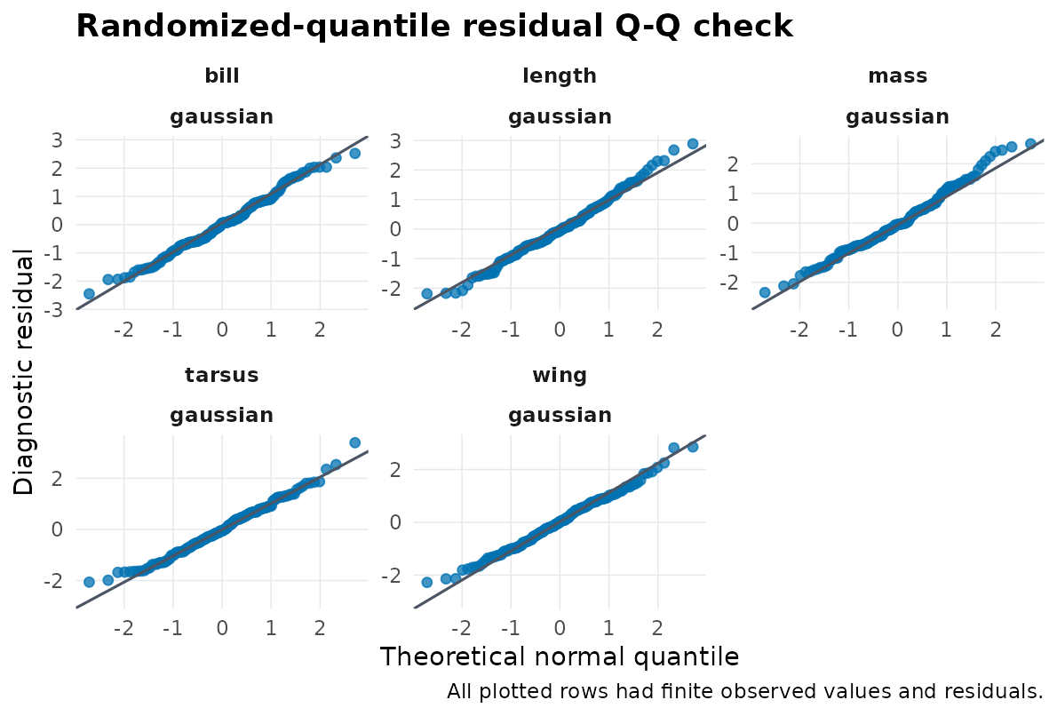
Marginal simulation-rank residual Q-Q check for the fitted Gaussian morphometrics model. New random effects are generated for each fitted-model draw. The plot is a diagnostic display, not interval calibration or a posterior predictive check.
Read the covariance summaries first
Start with the fitted Sigma rows. These rows describe
the covariance surface implied by the model, not a separate model:
sigma_rows <- extract_Sigma_table(fit, level = "unit")
sigma_rows
#>                     estimand trait_i trait_j i j level component matrix
#> 1  Sigma_unit[length,length]  length  length 1 1  unit     total  Sigma
#> 2    Sigma_unit[length,mass]  length    mass 1 2  unit     total  Sigma
#> 3      Sigma_unit[mass,mass]    mass    mass 2 2  unit     total  Sigma
#> 4    Sigma_unit[length,wing]  length    wing 1 3  unit     total  Sigma
#> 5      Sigma_unit[mass,wing]    mass    wing 2 3  unit     total  Sigma
#> 6      Sigma_unit[wing,wing]    wing    wing 3 3  unit     total  Sigma
#> 7  Sigma_unit[length,tarsus]  length  tarsus 1 4  unit     total  Sigma
#> 8    Sigma_unit[mass,tarsus]    mass  tarsus 2 4  unit     total  Sigma
#> 9    Sigma_unit[wing,tarsus]    wing  tarsus 3 4  unit     total  Sigma
#> 10 Sigma_unit[tarsus,tarsus]  tarsus  tarsus 4 4  unit     total  Sigma
#> 11   Sigma_unit[length,bill]  length    bill 1 5  unit     total  Sigma
#> 12     Sigma_unit[mass,bill]    mass    bill 2 5  unit     total  Sigma
#> 13     Sigma_unit[wing,bill]    wing    bill 3 5  unit     total  Sigma
#> 14   Sigma_unit[tarsus,bill]  tarsus    bill 4 5  unit     total  Sigma
#> 15     Sigma_unit[bill,bill]    bill    bill 5 5  unit     total  Sigma
#>     estimate lower upper interval_method interval_status  scale diagonal
#> 1  1.1813867    NA    NA            none            none latent     TRUE
#> 2  1.1327931    NA    NA            none            none latent    FALSE
#> 3  1.3287479    NA    NA            none            none latent     TRUE
#> 4  0.8660271    NA    NA            none            none latent    FALSE
#> 5  0.8621433    NA    NA            none            none latent    FALSE
#> 6  1.1448287    NA    NA            none            none latent     TRUE
#> 7  0.7652157    NA    NA            none            none latent    FALSE
#> 8  0.7383826    NA    NA            none            none latent    FALSE
#> 9  0.8852392    NA    NA            none            none latent    FALSE
#> 10 0.9995191    NA    NA            none            none latent     TRUE
#> 11 0.6693191    NA    NA            none            none latent    FALSE
#> 12 0.8040546    NA    NA            none            none latent    FALSE
#> 13 0.2984251    NA    NA            none            none latent    FALSE
#> 14 0.1790637    NA    NA            none            none latent    FALSE
#> 15 0.9340568    NA    NA            none            none latent     TRUE
#>    triangle
#> 1  diagonal
#> 2     upper
#> 3  diagonal
#> 4     upper
#> 5     upper
#> 6  diagonal
#> 7     upper
#> 8     upper
#> 9     upper
#> 10 diagonal
#> 11    upper
#> 12    upper
#> 13    upper
#> 14    upper
#> 15 diagonal
The full covariance target is stored in the example object, so this teaching example can show what the fitted model is trying to recover:
round(truth$Sigma, 2)
#>        length mass wing tarsus bill
#> length   0.97 0.92 0.68   0.58 0.60
#> mass     0.92 1.14 0.72   0.60 0.72
#> wing     0.68 0.72 1.00   0.76 0.24
#> tarsus   0.58 0.60 0.76   0.86 0.12
#> bill     0.60 0.72 0.24   0.12 0.90
Ordination of individuals on the two latent axes. These axes come from the fitted latent model (), not an eigen-decomposition of the raw data — this is model-based ordination, not PCA or NMDS:
ord <- extract_ordination(fit, level = "unit")
plot(ord$scores[, 1], ord$scores[, 2], pch = 19, col = "steelblue",
     xlab = "LV 1", ylab = "LV 2",
     main = "Individuals on latent trait axes")
abline(h = 0, v = 0, lty = 2, col = "grey70")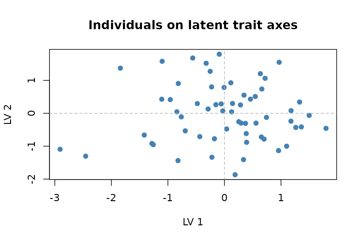
Individual scores on the two latent trait axes.
That’s the whole model — latent() for shared trait
covariance and the diagonal trait-specific
component, plus trait-specific intercepts.
Per-trait communality — the proportion of each trait’s variance shared with the others:
extract_communality(fit, "unit")
#>    length      mass      wing    tarsus      bill
#> 0.8911057 0.9348032 0.8055346 0.8684255 0.7801652
Pairwise trait correlations are point estimates by default. This is
the safest general summary because interval calibration depends on the
fitted target and model. method = "fisher-z" adds fast
heuristic bounds, while profile and bootstrap routes are slower and
remain target-specific rather than universally calibrated.
corr_rows <- extract_correlations(fit, tier = "unit")
corr_rows
#>    tier trait_i trait_j correlation lower upper method interval_status
#> 1     B  length    mass   0.9041350    NA    NA   none            none
#> 2     B  length    wing   0.7446723    NA    NA   none            none
#> 3     B    mass    wing   0.6990173    NA    NA   none            none
#> 4     B  length  tarsus   0.7041940    NA    NA   none            none
#> 5     B    mass  tarsus   0.6407146    NA    NA   none            none
#> 6     B    wing  tarsus   0.8275512    NA    NA   none            none
#> 7     B  length    bill   0.6371630    NA    NA   none            none
#> 8     B    mass    bill   0.7217348    NA    NA   none            none
#> 9     B    wing    bill   0.2885881    NA    NA   none            none
#> 10    B  tarsus    bill   0.1853213    NA    NA   none            none
For reports, plot the same tidy rows instead of hand-indexing a correlation matrix:
plot_correlations(corr_rows, sort = "magnitude")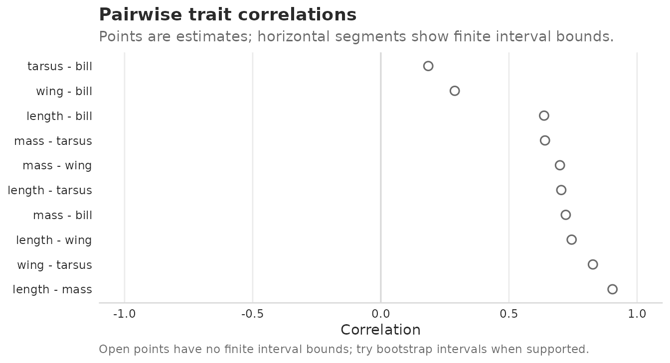
Pairwise point estimates of trait correlations from the first fitted model. No interval bounds are requested in this first-fit view.
The matrix form is a display over the same rows: the upper triangle
shows point estimates, and the lower triangle shows the finite Fisher-z
interval bounds supplied by extract_correlations(). The
plot does not compute or calibrate uncertainty itself.
plot_correlations(
  corr_rows,
  style = "heatmap",
  matrix_layout = "by_level",
  label_type = "estimate",
  title = "First-model trait correlations"
)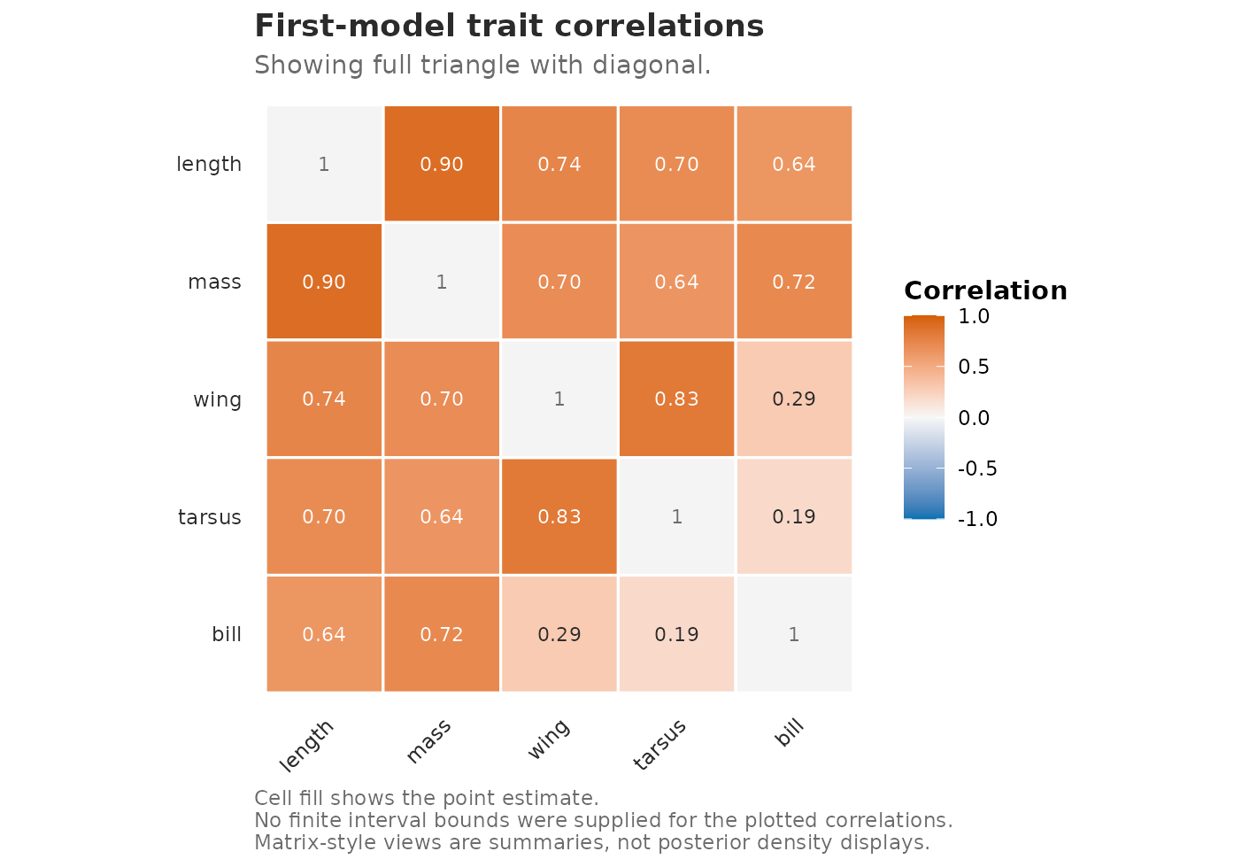
Point estimates of trait correlations from the first fitted model. The matrix is descriptive; interval routes are target-specific and opt-in.
Then inspect loadings and scores
The recovered loadings are useful, but they are not the first interpretation target. Only is identified directly from the data; raw loading columns can change sign or rotate.
Lambda_hat <- extract_loadings(fit, level = "unit")
rownames(Lambda_hat) <- paste0("trait_", seq_len(n_traits))
colnames(Lambda_hat) <- paste0("LV", seq_len(ncol(Lambda_hat)))
round(Lambda_hat, 3)
#>           LV1    LV2
#> trait_1 1.026  0.000
#> trait_2 1.104 -0.152
#> trait_3 0.844  0.458
#> trait_4 0.746  0.558
#> trait_5 0.652 -0.551
Do not over-interpret the signs of these unrotated loadings. Use them
as a quick look at the latent variables, then use Sigma,
correlations, and communality for report-ready interpretation unless you
have chosen a rotation or confirmatory constraint.
The shared covariance from the loadings can still be compared with
the known truth in this simulated teaching object. The off-diagonal
pattern is what should agree; the full Sigma diagonal also
includes Psi.
list(true_LL  = round(Lambda_true %*% t(Lambda_true), 2),
     fitted_LL = round(Lambda_hat  %*% t(Lambda_hat),  2))
#> $true_LL
#>        length mass wing tarsus bill
#> length   0.82 0.92 0.68   0.58 0.60
#> mass     0.92 1.04 0.72   0.60 0.72
#> wing     0.68 0.72 0.80   0.76 0.24
#> tarsus   0.58 0.60 0.76   0.74 0.12
#> bill     0.60 0.72 0.24   0.12 0.72
#>
#> $fitted_LL
#>         trait_1 trait_2 trait_3 trait_4 trait_5
#> trait_1    1.05    1.13    0.87    0.77    0.67
#> trait_2    1.13    1.24    0.86    0.74    0.80
#> trait_3    0.87    0.86    0.92    0.89    0.30
#> trait_4    0.77    0.74    0.89    0.87    0.18
#> trait_5    0.67    0.80    0.30    0.18    0.73
That is the whole first model: trait-specific intercepts, individual
latent scores, loadings from those scores to traits, and the diagonal
Psi carried by ordinary latent().
Choose your next guide
The next step depends on the question, not on adding every available model component:
- Interpret covariance: continue with Individual morphometrics for a fuller Gaussian worked example.
- Check the fit: use Can I trust this fit? before relying on coefficients, covariance, or uncertainty.
- Choose a specialised model: use the Articles chooser to select repeated behaviours, reaction norms, binary occurrence, phylogenetic covariance, missing data, rank selection, or a technical reference.
Family, grouping structure, covariance source, covariance mode, missingness, and latent rank answer different scientific questions. Add only the pieces the sampling design and estimand require.
Acknowledgements
gllvmTMB is a standalone TMB-based package. Its design
borrows ideas from several earlier projects, whose corresponding GPL-3
code is incorporated and whose authors are credited in
DESCRIPTION (as copyright holders) and listed in
inst/COPYRIGHTS:
- sdmTMB (Anderson, Ward, English, Barnett, Thorson, et al.): sparse SPDE / GMRF spatial machinery.
-
glmmTMB
(Brooks, Bolker, Kristensen, Magnusson, Skaug, Nielsen, Berg, van
Bentham, et al.):
rr/propto/equalto/diagcovariance dispatch. The reduced-rankrr()machinery in particular is the contribution of McGillycuddy, Popovic, Bolker & Warton (2025) J. Stat. Softw. 112(1). -
GALAMM
(Sørensen): mixed-response (
gfam) and confirmatory fixed-loading (lambda_constraint) patterns. -
MCMCglmm
(Hadfield): sparse
phylogeny representation used by
phylo_latent(). - TMB (Kristensen et al.) and fmesher (Lindgren): autodiff and finite-element mesh.