Joint species distribution models for binary occurrence data

After an environmental gradient is in the model, which species still tend to occur together, and which species avoid each other? That is the first joint species distribution model (JSDM) question this page answers.

The data are binary occurrence records: one row per site, one column or trait per species, and a 0/1 response for absence/presence. The model uses latent() to estimate a low-rank residual co-occurrence structure across species after env_1 is accounted for.

This example supports both long data and the wide traits(...) formula, using a binomial-logit model with latent(0 + trait | site, d = K) for residual co-occurrence. The Fisher-z intervals below are model-based uncertainty diagnostics; their repeated-sampling coverage has not been established for this model class. Single-species spatial SDMs belong in sdmTMB, and multivariate spatial fields via spatial_*() are beyond the scope of this introductory JSDM example.

Setup

library(gllvmTMB)
library(ggplot2)

Load and fit

The article uses a shipped teaching fixture rather than building the data inside the vignette. It contains a complete Site x Species occurrence matrix: 120 sites, 8 species, 2 latent residual co-occurrence axes, and an environmental covariate env_1 with species-specific responses. The true loadings put the species into four niche quadrants (dry-low, dry-high, wet-low, wet-high), with two species per quadrant.

jsdm_path <- system.file(
  "extdata", "examples", "joint-sdm-example.rds",
  package = "gllvmTMB"
)

source_candidates <- file.path(
  c(".", "..", "../.."),
  "inst", "extdata", "examples", "joint-sdm-example.rds"
)
input_file <- knitr::current_input(dir = TRUE)
if (!is.null(input_file)) {
  source_candidates <- c(
    source_candidates,
    file.path(
      dirname(dirname(dirname(input_file))),
      "inst", "extdata", "examples", "joint-sdm-example.rds"
    )
  )
}
candidate_paths <- c(jsdm_path, source_candidates)
candidate_paths <- candidate_paths[nzchar(candidate_paths)]
jsdm_path <- candidate_paths[file.exists(candidate_paths)][1]
if (is.na(jsdm_path)) {
  stop("Could not find joint-sdm-example.rds.")
}
jsdm <- readRDS(jsdm_path)

df <- jsdm$data_long
df_wide <- jsdm$data_wide

The same JSDM fits in both long format and the traits(...) wide format. The long form is shown first; the wide form is the formula-API equivalent on a pivoted data frame. Both reach the same engine.

# Long format -- one row per (site, species) observation
fit_jsdm <- gllvmTMB(
  value ~ 0 + trait + (0 + trait):env_1 +
    latent(0 + trait | site, d = 2),
  data   = df,
  trait  = "trait",
  unit   = "site",
  family = binomial()
)
fit_jsdm
#> Stacked-trait gllvmTMB fit
#>   Traits = 8, site = 120 
#>   Covstructs: latent_unit, indep_unit 
#>   Fixed effects (b_fix): 16
#>   ML log L = 11765.408   convergence = 0
#>   Note: Lambda_B identified up to rotation (use suggest_lambda_constraint() or rotate_loadings()).
#>   Run gllvmTMB_diagnose(fit) for a full health check, or summary(fit) for parameter estimates.

# Wide format -- one row per site, one column per species. The
# `traits(...)` LHS names the species columns; the compact RHS
# shorthand uses `1 + env_1`, which expands internally to
# `0 + trait + (0 + trait):env_1`.
fit_jsdm_wide <- gllvmTMB(
  traits(sp_1, sp_2, sp_3, sp_4, sp_5, sp_6, sp_7, sp_8) ~
    1 + env_1 + latent(1 | site, d = 2),
  data   = df_wide,
  unit   = "site",
  family = binomial()
)
all.equal(logLik(fit_jsdm), logLik(fit_jsdm_wide), tolerance = 1e-8)
#> [1] TRUE

Long or wide data shape

JSDM is the package’s natural long-format use case because each row already carries (site, species) and the response factor trait indexes species. When the data already live as one row per site and one binary column per species, the traits(...) wide form is the same model through the same gllvmTMB() entry point. In either shape, true absences should be explicit zeros. Missing response cells are not a safe shortcut for absences, because missingness can also mean the site or species was not surveyed.

What latent() estimates

For binary occurrence data with a logit link, the fitted linear predictor is

$$\mathrm{logit}\{P(y_{it} = 1)\} = \mathbf x_i^\top \boldsymbol\beta_t + \boldsymbol\lambda_t^\top \mathbf u_i, \qquad \mathbf u_i \sim \mathcal N(\mathbf 0, \mathbf I_d).$$

The site score $\mathbf u_i$ is the unobserved residual state of site $i$, and the species loading $\boldsymbol\lambda_t$ says how species $t$ responds to those residual axes. The rotation of $\boldsymbol\Lambda$ is arbitrary, so the stable co-occurrence target is the species covariance implied by the loadings. For this single-trial Bernoulli fixture, each species-site cell contributes one binary observation. The default between-site diagonal companion is therefore not separately identified from the link scale and the engine maps it off:

$$\boldsymbol\Sigma_B = \boldsymbol\Lambda\boldsymbol\Lambda^\top.$$

For a binary logit JSDM, correlations are easier to interpret on the latent-liability scale. extract_correlations(link_residual = "auto") adds the fixed logistic residual variance $\pi^2 / 3$ to the diagonal:

$$\boldsymbol\Sigma_{\mathrm{latent}} = \boldsymbol\Lambda\boldsymbol\Lambda^\top + (\pi^2 / 3)\mathbf I.$$

The logistic residual term is fixed by the binomial logit link, not estimated from the data. Ordinary latent() normally carries a diagonal $\boldsymbol\Psi_B$ companion, but the fit message explains why that default component is mapped off for these single-trial cells. Multi-trial binomial data or genuine repeated observations can identify additional variation; they are different designs and should not be inferred from this occurrence matrix.

Where loading constraints fit

The loading matrix $\boldsymbol\Lambda$ is usually exploratory in a JSDM: its rotation is arbitrary, while $\boldsymbol\Lambda\boldsymbol\Lambda^\top$ is the interpretable co-occurrence target. If you have an a-priori hypothesis that a species group defines an axis, or that a species should have zero loading on an axis, that is a confirmatory loading question rather than the default species-distribution workflow.

gllvmTMB supports that confirmatory path with lambda_constraint = list(unit = M), where NA means “estimate this loading” and a number means “pin this loading during fitting.” Numeric pins are exact model restrictions: because the latent scores have unit variance, a loading pinned to 1 is assumed to equal one; it is not a cosmetic sign convention. The current route acts on the packed lower-triangular loading matrix, so it is not a general free-form confirmatory-factor interface.

Specify a biological loading hypothesis before inspecting this fitted loading matrix, verify that the matrix rows follow the response order, and stop if the constrained fit is unhealthy. A matrix suggested from the same data can provide a reproducible descriptive orientation, but it remains exploratory and does not turn selected zeros into biological facts. This guide therefore keeps correlations and $\boldsymbol\Sigma$ as its interpretation targets.

Latent-scale residual species correlations

Pairwise species correlations on the latent-liability scale. The opt-in method = "fisher-z" gives Fisher-transform heuristic bounds that are fast (seconds) and bounded inside $[-1, 1]$ by construction. method = "wald" is an accepted alias for the same Fisher-z path. Two heavier alternatives are also available: method = "bootstrap" re-fits the model under a parametric bootstrap for a full sampling-distribution CI, and method = "profile" inverts the profile likelihood pair-by-pair (cost scales as $O(T(T-1)/2)$ constrained refits).

One scale caveat is worth stating up front, because it trips people up on binary fits. The default link_residual = "auto" puts the correlation on the latent-liability scale — it adds the fixed logistic residual $\pi^2/3$ to the diagonal of $\boldsymbol\Sigma_B$ before forming the correlation, which is the interpretable co-occurrence quantity for a JSDM. fisher-z, wald, and bootstrap all honour that argument. The current profile path, however, always reports the correlation of the bare $\boldsymbol\Sigma_B = \boldsymbol\Lambda\boldsymbol\Lambda^\top$ (it ignores link_residual), so its point estimate is the undiluted latent-factor correlation, not the latent-liability one. The optional comparison snippets below make the difference explicit for readers who want to audit the scale.

What is and is not certified: the point estimates and Fisher-z bounds are useful diagnostics for this fitted example, but the package-wide calibrated-coverage work is still open. Treat intervals here as model-based uncertainty summaries, not as a claim that every binary or mixed-family covariance interval has reached nominal coverage.

corr_rows <- extract_correlations(
  fit_jsdm,
  tier = "unit",
  method = "fisher-z",
  link_residual = "auto"
)
corr_rows
#>    tier trait_i trait_j  correlation       lower       upper   method
#> 1     B    sp_1    sp_2  0.153555913 -0.02641239  0.32388284 fisher-z
#> 2     B    sp_1    sp_3  0.128632141 -0.05180359  0.30093506 fisher-z
#> 3     B    sp_2    sp_3  0.018398708 -0.16137481  0.19699041 fisher-z
#> 4     B    sp_1    sp_4 -0.038128913 -0.21589477  0.14208346 fisher-z
#> 5     B    sp_2    sp_4 -0.093762798 -0.26849182  0.08693966 fisher-z
#> 6     B    sp_3    sp_4  0.153546600 -0.02642192  0.32387430 fisher-z
#> 7     B    sp_1    sp_5 -0.028984725 -0.20714987  0.15104131 fisher-z
#> 8     B    sp_2    sp_5  0.072350398 -0.10829533  0.24837082 fisher-z
#> 9     B    sp_3    sp_5 -0.288700390 -0.44491851 -0.11543233 fisher-z
#> 10    B    sp_4    sp_5 -0.197555473 -0.36391070 -0.01898645 fisher-z
#> 11    B    sp_1    sp_6 -0.115408285 -0.28867805  0.06518139 fisher-z
#> 12    B    sp_2    sp_6 -0.044896452 -0.22234849  0.13543477 fisher-z
#> 13    B    sp_3    sp_6 -0.209613817 -0.37477434 -0.03155816 fisher-z
#> 14    B    sp_4    sp_6 -0.077285072 -0.25302139  0.10338847 fisher-z
#> 15    B    sp_5    sp_6  0.168001108 -0.01158921  0.33709169 fisher-z
#> 16    B    sp_1    sp_7 -0.140516818 -0.31190245  0.03972505 fisher-z
#> 17    B    sp_2    sp_7 -0.164262535 -0.33367947  0.01543320 fisher-z
#> 18    B    sp_3    sp_7  0.054151117 -0.12631626  0.23114890 fisher-z
#> 19    B    sp_4    sp_7  0.139373438 -0.04088938  0.31084930 fisher-z
#> 20    B    sp_5    sp_7 -0.146835893 -0.31771526  0.03328138 fisher-z
#> 21    B    sp_6    sp_7  0.001381071 -0.17790431  0.18057771 fisher-z
#> 22    B    sp_1    sp_8 -0.202881734 -0.36871483 -0.02453251 fisher-z
#> 23    B    sp_2    sp_8 -0.201163228 -0.36716576 -0.02274189 fisher-z
#> 24    B    sp_3    sp_8 -0.023443364 -0.20183658  0.15645540 fisher-z
#> 25    B    sp_4    sp_8  0.124534776 -0.05595559  0.29714335 fisher-z
#> 26    B    sp_5    sp_8 -0.096574066 -0.27112226  0.08412346 fisher-z
#> 27    B    sp_6    sp_8  0.058834221 -0.12169041  0.23559113 fisher-z
#> 28    B    sp_7    sp_8  0.217567191  0.03988110  0.38191498 fisher-z
#>          interval_status
#> 1  heuristic_unvalidated
#> 2  heuristic_unvalidated
#> 3  heuristic_unvalidated
#> 4  heuristic_unvalidated
#> 5  heuristic_unvalidated
#> 6  heuristic_unvalidated
#> 7  heuristic_unvalidated
#> 8  heuristic_unvalidated
#> 9  heuristic_unvalidated
#> 10 heuristic_unvalidated
#> 11 heuristic_unvalidated
#> 12 heuristic_unvalidated
#> 13 heuristic_unvalidated
#> 14 heuristic_unvalidated
#> 15 heuristic_unvalidated
#> 16 heuristic_unvalidated
#> 17 heuristic_unvalidated
#> 18 heuristic_unvalidated
#> 19 heuristic_unvalidated
#> 20 heuristic_unvalidated
#> 21 heuristic_unvalidated
#> 22 heuristic_unvalidated
#> 23 heuristic_unvalidated
#> 24 heuristic_unvalidated
#> 25 heuristic_unvalidated
#> 26 heuristic_unvalidated
#> 27 heuristic_unvalidated
#> 28 heuristic_unvalidated

The matrix view below shows the same point estimates as a species-by-species map. For a binary JSDM, the useful first picture is the latent-liability correlation pattern after adding the fixed logistic link residual to the denominator; raw $\boldsymbol\Sigma_B$ entries can be dominated by loading scale and are harder to interpret. The Fisher-z interval bounds stay in corr_rows rather than being printed inside every matrix cell.

plot_correlations(
  corr_rows,
  style = "heatmap",
  matrix_layout = "by_level",
  label_type = "estimate",
  label_digits = 2,
  include_diagonal = TRUE,
  title = "Residual species correlations",
  subtitle = "Latent-liability correlations after accounting for env_1."
) +
  ggplot2::labs(caption = NULL)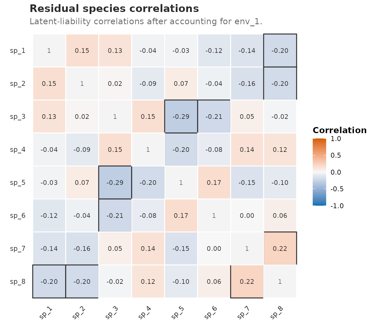

Residual species correlations from the fitted binary JSDM. Cells show Fisher-z point estimates on the latent-liability scale after accounting for env_1 and the fixed logistic link residual; interval bounds are available in the preceding table.

Use these correlations, rather than the signs of individual loadings, for the rotation-invariant co-occurrence story.

Confidence intervals on the binary latent scale

This section works through the three CI methods on two estimands — a pairwise species correlation and a per-species ICC — to show what each method returns and where it currently stops short. These chunks are optional because the bootstrap and profile paths re-fit the model; run them when the interval method itself is the question, not for a first pass through the article.

Three CI methods for one correlation

Take a single species pair (sp_1, sp_2) and ask for the same correlation three ways. Keeping link_residual = "auto" for the Fisher-z and bootstrap calls holds them on the latent-liability scale, so their point estimates agree and only the interval differs:

pair_ij <- c("sp_1", "sp_2")

cor_fisher <- extract_correlations(
  fit_jsdm, tier = "unit", pair = pair_ij,
  method = "fisher-z", link_residual = "auto"
)
cor_boot <- extract_correlations(
  fit_jsdm, tier = "unit", pair = pair_ij,
  method = "bootstrap", nsim = 20, seed = 1, link_residual = "auto"
)
rbind(cor_fisher, cor_boot)[, c("trait_i", "trait_j",
                                "correlation", "lower", "upper", "method")]

The Fisher-z and bootstrap point estimates match because both add the $\pi^2/3$ logistic residual to the diagonal; the bootstrap interval is the empirical 2.5/97.5 percentile across the refits.

The profile method is the one that reports a different number, because it currently works on the bare $\boldsymbol\Sigma_B$ scale. To compare it fairly, request the Fisher-z interval with link_residual = "none" so both sit on the same (undiluted) scale:

cor_profile <- extract_correlations(
  fit_jsdm, tier = "unit", pair = pair_ij,
  method = "profile"
)
cor_fisher_bare <- extract_correlations(
  fit_jsdm, tier = "unit", pair = pair_ij,
  method = "fisher-z", link_residual = "none"
)
rbind(cor_profile, cor_fisher_bare)[, c("trait_i", "trait_j",
                                        "correlation", "lower", "upper", "method")]

Now the two point estimates agree: the profile correlation matches the bare-scale Fisher-z value. The profile interval is a likelihood-ratio inversion around that point — but note it can come back as NA when the constrained refit fails to bracket the bound (a near-boundary correlation here is a common cause), which is the same not-yet-calibrated CI story flagged above. The take-home is not that one method is wrong, but that profile and the default latent-liability correlations live on different scales until the profile path learns to honour link_residual. For the interpretable JSDM co-occurrence story, prefer the latent-liability scale (auto), and use Fisher-z for speed or the bootstrap when you want an empirical sampling-distribution interval.

ICC (communality) on the latent scale

For a single-trial binary JSDM, the natural communality quantity is the share of each species’ latent-liability variance represented by the shared factors rather than the fixed logistic residual:

$$\mathrm{ICC}_t \;=\; \frac{(\boldsymbol\Lambda\boldsymbol\Lambda^\top)_{tt}} {(\boldsymbol\Lambda\boldsymbol\Lambda^\top)_{tt} + \pi^2/3}.$$

The unit-level latent() term estimates the shared loading covariance, and link_residual = "auto" adds the fixed logistic residual variance $\pi^2/3$, so extract_communality(level = "unit", link_residual = "auto") returns exactly this ratio — the proportion of the latent-liability variance that the shared factors explain. (This is not the between-vs-within extract_repeatability() ICC, which needs paired between- and within-unit diagonal tiers such as indep(0 + trait | site) + indep(0 + trait | site_species); a single-trial occurrence matrix has no within-site replication for that, so extract_repeatability() and extract_ICC_site() are not applicable to this fit.)

icc_point <- extract_communality(
  fit_jsdm, level = "unit", link_residual = "auto"
)
round(icc_point, 3)
#>  sp_1  sp_2  sp_3  sp_4  sp_5  sp_6  sp_7  sp_8 
#> 0.193 0.152 0.323 0.143 0.310 0.143 0.195 0.266

A parametric bootstrap puts an interval on each species’ ICC:

icc_boot <- extract_communality(
  fit_jsdm, level = "unit", link_residual = "auto",
  ci = TRUE, method = "bootstrap", nsim = 20, seed = 1
)
icc_boot[, c("trait", "c2", "lower", "upper", "method")]

The intervals are wide — eight species and 120 sites is modest information for a per-species variance share, and the upper bounds for the more strongly-loading species run close to 1.

Two limitations apply to the ICC interval in this example:

• Wald is not implemented for communality (it is a non-linear function of several parameters); requesting method = "wald" emits a note and falls back to the bootstrap.
• Profile bounds are not yet delivered for this proportion on a single-trial binary fit — the constrained refit fails to bracket and the interval returns NA. The point estimate is still the correct latent-scale ICC; only the profile interval is missing.

The point estimates are available, but interval coverage on binary and mixed-family scales has not been established. Report the point estimate and the interval method used; do not present these intervals as coverage-certified.

Ordination biplot

Site scores on the two latent variables (LV1, LV2), with species loadings shown as arrows. This is model-based ordination: LV1 and LV2 are the latent variables of a fitted GLLVM, estimated jointly with the env_1 regression — not a variance-maximising PCA, a distance-based NMDS embedding, or a covariate-constrained CCA/RDA of the raw occurrence matrix. The plotted site scores are predicted (empirical-Bayes) conditional modes of the residual site states $u_i$: shrunk toward zero, and carrying prediction uncertainty the point display does not show. The rotation-invariant interpretation target is the model-implied residual co-occurrence $\boldsymbol\Sigma_B$ (defined above), not the axis coordinates themselves — species loading in the same direction tend to co-occur after env_1 is accounted for.

plot(
  fit_jsdm,
  type = "ordination",
  level = "unit",
  rotation = "varimax",
  sign_anchor = "auto",
  standardize_loadings = TRUE
) +
  ggplot2::labs(
    title = "Residual species ordination",
    subtitle = "Varimax-rotated site scores and species loading directions.",
    caption = NULL
  )

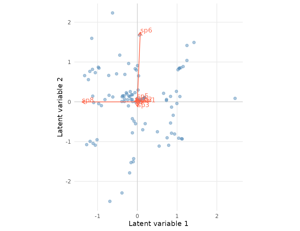
Ordination biplot from the fitted binary JSDM, using varimax-rotated and sign-anchored site scores and species loadings. Loading orientation and sign are not identifiable; the model-implied Sigma and correlations remain the rotation-invariant interpretation target.

The fixture’s truth places the eight species into four designed association groups: sp_1 / sp_2, sp_3 / sp_4, sp_5 / sp_6, and sp_7 / sp_8. The fitted arrows should be read for broad grouping, not axis labels. The exact orientation is arbitrary — only $\boldsymbol\Lambda\boldsymbol\Lambda^\top$ is identifiable. Species arrows pointing in the same direction co-occur after env_1 is accounted for; arrows pointing in opposite directions tend to mutually exclude.

See also

• Morphometrics — Gaussian stacked-trait analogue with ordinary latent().
• Choosing latent rank — how to compare candidate values of d.
• Loading-constraint helpers — ?confirmatory_lambda and ?suggest_lambda_constraint document the advanced API contracts.
• vignette("response-families") — full table of supported families and the per-family $\sigma^2_d$.

References

• Niku, J., Warton, D.I., Hui, F.K.C., & Taskinen, S. (2017). Generalized linear latent variable models for multivariate count and biomass data in ecology. Journal of Agricultural, Biological, and Environmental Statistics 22, 498–522. https://link.springer.com/article/10.1007/s13253-017-0304-7
• Niku, J., Hui, F.K.C., Taskinen, S., & Warton, D.I. (2019). gllvm: Fast analysis of multivariate abundance data with generalized linear latent variable models in r. Methods in Ecology and Evolution 10, 2173–2182. https://doi.org/10.1111/2041-210X.13303
• Nakagawa, S., & Schielzeth, H. (2010). Repeatability for Gaussian and non-Gaussian data: a practical guide for biologists. Biological Reviews 85, 935–956. https://doi.org/10.1111/j.1469-185X.2010.00141.x
• Nakagawa, S., Johnson, P.C.D., & Schielzeth, H. (2017). The coefficient of determination R² and intra-class correlation coefficient from generalized linear mixed-effects models revisited and expanded. Journal of the Royal Society Interface 14,
  20170213. https://doi.org/10.1098/rsif.2017.0213
• Warton, D.I., Blanchet, F.G., O’Hara, R.B., Ovaskainen, O., Taskinen, S., Walker, S.C., & Hui, F.K.C. (2015). So many variables: joint modeling in community ecology. Trends in Ecology & Evolution 30, 766–779. https://doi.org/10.1016/j.tree.2015.09.007