Cross-lineage covariance in a plant--bumblebee example

This article shows the smallest cross-lineage phylogenetic workflow: flower traits from one lineage and bumblebee traits from another share a supplied, association-derived kernel. The output is a plant-trait by bumblebee-trait covariance block, not an interaction model.

Synthetic teaching data. Every species name, trait value, phylogeny, and interaction weight below was simulated for this article. The names make the workflow concrete; they are not observations from a real plant–bumblebee network. A suitable public empirical source is the CC0 data record of Liang (2020, Dryad); substituting it requires deliberate species-name and trait checks before fitting.

Evidence boundary. This is a fixed-rho, Gaussian point-estimate example. rho is supplied when the kernel is built, not estimated by the model. The covariance block has no calibrated interval here, and it is not evidence that traits causally coevolved. Sparse association data, a different defensible rho, or a different interaction matrix can change the result.

Scope boundary. In: one named, dense kernel_latent() tier and its shared plant-by-bumblebee covariance block. Partial: the fixed-rho point estimate demonstrated here; it is sensitive to the supplied kernel and association matrix. Not provided: estimated rho, calibrated intervals, a causal coevolution test, or a separately interpreted phylogenetic-versus-tip decomposition.

Engine note. Run this example with engine = "tmb" (the default). The current engine = "julia" bridge deliberately does not route kernel_latent() or other structured covariance terms. GLLVModels.jl has a Gaussian dense-covariance building block, but the R bridge has not yet been validated to represent this kernel-only model or return its named covariance component.

The model and its estimand

Let (A_F) and (A_B) be fixed plant and bumblebee phylogenetic correlation matrices, and let (W) be the observed or assumed plant-by-bumblebee association matrix. make_cross_kernel() builds a positive-semidefinite stacked kernel

$$K_{\mathrm{cross}} = \begin{bmatrix} A_F & C_{FB} \\ C_{FB}^{\mathsf T} & A_B \end{bmatrix},$$

where the off-diagonal block (C_{FB}) is a spectrally scaled function of (A_F), (A_B), (W), and the fixed bridge strength ( ho). A latent Gaussian field (G (0, K_{})) then gives

$$Y = M + G\Lambda^{\mathsf T} + E, \qquad \Gamma_{FB} = \Lambda_F\Lambda_B^{\mathsf T}.$$

Gamma is the block whose rows are flower traits and whose columns are bumblebee traits. It summarizes the fitted shared covariance shape conditional on the supplied kernel. It does not identify a mechanism, establish the direction of evolutionary change, or turn the interaction matrix into a response variable.

Symbol in prose	Keyword or helper	Teaching-data draw	Extractor	Known teaching value
(K_{})	make_cross_kernel()	fixed from (A_F, A_B, W, )	eigenvalue and name checks	example$K_cross
(G)	kernel_latent(..., d = 2, name = "cross")	((0, K_{}))	extract_Sigma(..., part = "shared")	Lambda %*% t(Lambda)
(Gamma_{FB})	same named kernel tier	Lambda_plant %*% t(Lambda_bumblebee)	extract_Gamma()	example$truth$Gamma

Load the synthetic plant–bumblebee fixture

library(gllvmTMB)
library(ggplot2)

example_path <- system.file(
  "extdata", "examples", "plant-bumblebee-coevolution-example.rds",
  package = "gllvmTMB"
)
example_path <- c(
  example_path,
  file.path("inst", "extdata", "examples", "plant-bumblebee-coevolution-example.rds"),
  file.path("..", "inst", "extdata", "examples", "plant-bumblebee-coevolution-example.rds"),
  file.path("..", "..", "inst", "extdata", "examples", "plant-bumblebee-coevolution-example.rds")
)
example_path <- example_path[nzchar(example_path) & file.exists(example_path)][1]
stopifnot(!is.na(example_path))
example <- readRDS(example_path)

theme_article <- function() {
  theme_minimal(base_size = 11) +
    theme(
      panel.grid.minor = element_blank(),
      panel.grid.major = element_line(colour = "#D9E2EC", linewidth = 0.28),
      plot.title = element_text(face = "bold", colour = "#102A43"),
      plot.subtitle = element_text(colour = "#486581"),
      plot.caption = element_text(colour = "#627D98", hjust = 0),
      axis.title = element_text(face = "bold", colour = "#243B53"),
      axis.text = element_text(colour = "#243B53"),
      legend.title = element_text(face = "bold", colour = "#243B53"),
      legend.position = "bottom"
    )
}

matrix_long <- function(x, row_name, col_name, value_name) {
  out <- as.data.frame(as.table(x), stringsAsFactors = FALSE)
  names(out) <- c(row_name, col_name, value_name)
  out
}

c(
  plants = example$truth$n_plant,
  bumblebees = example$truth$n_bumblebee,
  repeated_measurements = example$truth$n_replicate
)
#>                plants            bumblebees repeated_measurements 
#>                    12                     8                     6
head(example$data_wide)
#>       observation  species lineage flower_tube_depth nectar_volume
#> 1 observation_001 plant_01   plant          1.146396      1.285014
#> 2 observation_002 plant_01   plant          1.294460      1.046325
#> 3 observation_003 plant_01   plant          1.418918      1.198860
#> 4 observation_004 plant_01   plant          1.104701      1.225622
#> 5 observation_005 plant_01   plant          1.237340      1.036584
#> 6 observation_006 plant_01   plant          1.289209      1.205648
#>   tongue_length body_size
#> 1            NA        NA
#> 2            NA        NA
#> 3            NA        NA
#> 4            NA        NA
#> 5            NA        NA
#> 6            NA        NA

Each plant row has two observed flower traits and missing bumblebee traits; each bumblebee row has the complementary pattern. That block-missing layout is intentional. The model learns covariance across the two lineages through the supplied cross-kernel, not by pretending a plant has a tongue length.

Example 1: start with an association map, then build one kernel

The association matrix is an input that says which plant–bumblebee links are more prominent in this teaching system. It is not a response, a causal graph, or a discovery made by the fitted model. In an empirical analysis it should be constructed and justified before fitting, rather than tuned until a preferred trait pattern appears.

association_long <- matrix_long(
  example$W,
  row_name = "plant_species",
  col_name = "bumblebee_species",
  value_name = "association_weight"
)

ggplot(association_long, aes(bumblebee_species, plant_species,
  fill = association_weight)) +
  geom_tile(colour = "white", linewidth = 0.35) +
  scale_fill_viridis_c(
    option = "C", end = 0.9,
    name = "Supplied\nassociation weight"
  ) +
  labs(
    title = "The association map is declared before model fitting",
    subtitle = "Fictional plant--bumblebee links in the synthetic teaching fixture",
    x = "Bumblebee species", y = "Plant species"
  ) +
  theme_article() +
  theme(axis.text.x = element_text(angle = 35, hjust = 1))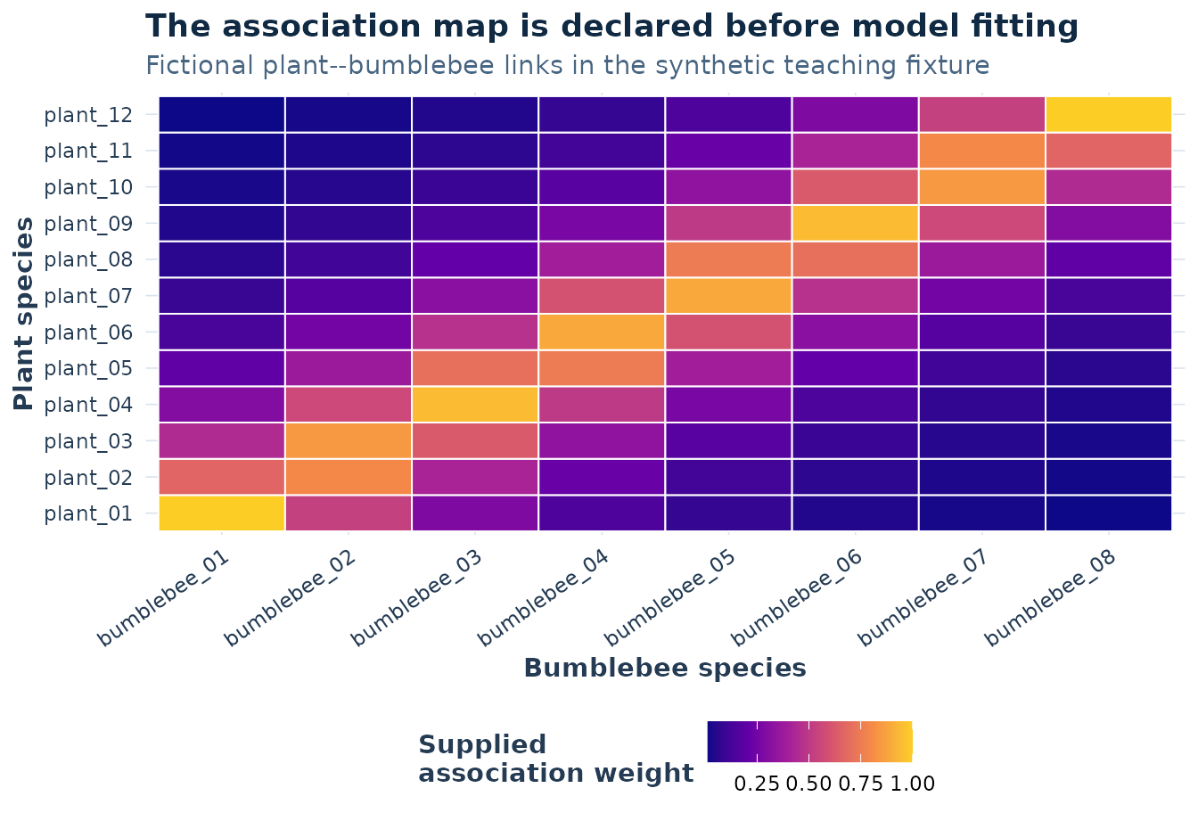

Synthetic association map used as the fixed input W. Darker tiles denote larger supplied association weights; the colours are not fitted probabilities.

Build and check the fixed cross-lineage kernel

K_cross <- make_cross_kernel(
  example$A_plant,
  example$A_bumblebee,
  example$W,
  rho = example$truth$rho
)

kernel_check <- list(
  reconstructed_exactly = isTRUE(all.equal(K_cross, example$K_cross)),
  minimum_eigenvalue = min(eigen(K_cross, symmetric = TRUE, only.values = TRUE)$values),
  plant_names_match = identical(rownames(example$A_plant), rownames(example$W)),
  bumblebee_names_match = identical(colnames(example$A_bumblebee), colnames(example$W))
)
kernel_check
#> $reconstructed_exactly
#> [1] TRUE
#> 
#> $minimum_eigenvalue
#> [1] 0.005660774
#> 
#> $plant_names_match
#> [1] TRUE
#> 
#> $bumblebee_names_match
#> [1] TRUE

The association map is transformed into a cross-lineage bridge only after the tree labels and matrix order agree. The bridge below is the plant-by-bumblebee off-diagonal block of the resulting kernel; its sign and scale are determined by the declared kernel construction and fixed rho.

n_plant <- example$truth$n_plant
kernel_bridge <- K_cross[
  seq_len(n_plant),
  n_plant + seq_len(example$truth$n_bumblebee),
  drop = FALSE
]
rownames(kernel_bridge) <- rownames(example$A_plant)
colnames(kernel_bridge) <- rownames(example$A_bumblebee)
kernel_bridge_long <- matrix_long(
  kernel_bridge,
  row_name = "plant_species",
  col_name = "bumblebee_species",
  value_name = "kernel_bridge"
)

ggplot(kernel_bridge_long, aes(bumblebee_species, plant_species,
  fill = kernel_bridge)) +
  geom_tile(colour = "white", linewidth = 0.35) +
  scale_fill_viridis_c(
    option = "B", end = 0.88,
    name = "Fixed kernel\nbridge"
  ) +
  labs(
    title = "The supplied association map becomes a fixed covariance bridge",
    subtitle = paste0("Kernel built with fixed rho = ", example$truth$rho),
    x = "Bumblebee species", y = "Plant species"
  ) +
  theme_article() +
  theme(axis.text.x = element_text(angle = 35, hjust = 1))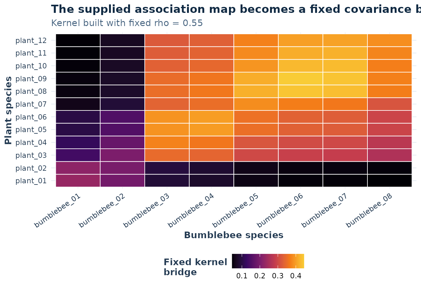

The plant-by-bumblebee bridge in the fixed cross-lineage kernel. This is an input covariance structure, not a fitted trait covariance block.

For real data, stop here if a species is absent from either tree, if names are duplicated across the two lineages, or if the interaction matrix is ordered differently from the trees. Prune and reorder deliberately, then rebuild the kernel. Do not repair those problems by relying on factor order.

Example 2: fit the shared plant–bumblebee trait block

The wide form has one observation per row and the four traits in columns. It is compact when the two sets of traits are already stored separately.

fit <- gllvmTMB(
  traits(flower_tube_depth, nectar_volume, tongue_length, body_size) ~ 1 +
    kernel_latent(species, K = K_cross, d = 2, name = "cross"),
  data = example$data_wide,
  unit = "observation",
  cluster = "species",
  family = gaussian(),
  control = gllvmTMBcontrol(se = FALSE)
)

c(
  convergence = fit$opt$convergence,
  log_likelihood = as.numeric(logLik(fit))
)
#>    convergence log_likelihood 
#>        0.00000       79.43296

The long form is equivalent in meaning and is often easier to construct from field data. It uses the same gllvmTMB() entry point:

fit_long <- gllvmTMB(
  value ~ 0 + trait +
    kernel_latent(species, K = K_cross, d = 2, name = "cross"),
  data = example$data_long,
  trait = "trait",
  unit = "observation",
  cluster = "species",
  family = gaussian(),
  control = gllvmTMBcontrol(se = FALSE)
)

Here the optimizer reached its normal convergence code. That is a numerical health check, not validation of an evolutionary conclusion; inspect check_gllvmTMB(fit) before interpreting a real fit.

Read the plant-by-bumblebee covariance block

Gamma_shape <- extract_Gamma(
  fit,
  level = "cross",
  row_traits = example$truth$plant_traits,
  col_traits = example$truth$bumblebee_traits,
  scale = "shape"
)
round(Gamma_shape, 3)
#>                   tongue_length body_size
#> flower_tube_depth         0.628    -0.705
#> nectar_volume             0.623    -0.279

The signs and relative sizes describe the fitted shared covariance shape for this synthetic draw, conditional on the chosen kernel. They are not estimates of a universal flower–pollinator matching rule. scale = "effect" would multiply this shape by the fixed rho; it would still not estimate rho.

gamma_long <- matrix_long(
  Gamma_shape,
  row_name = "flower_trait",
  col_name = "bumblebee_trait",
  value_name = "covariance_shape"
)
gamma_limit <- max(abs(gamma_long$covariance_shape))
gamma_long$label_colour <- ifelse(
  abs(gamma_long$covariance_shape) > 0.45 * gamma_limit,
  "white", "#102A43"
)
trait_labels <- c(
  flower_tube_depth = "Flower tube depth",
  nectar_volume = "Nectar volume",
  tongue_length = "Tongue length",
  body_size = "Body size"
)
gamma_long$flower_trait <- unname(trait_labels[gamma_long$flower_trait])
gamma_long$bumblebee_trait <- unname(trait_labels[gamma_long$bumblebee_trait])

ggplot(gamma_long, aes(bumblebee_trait, flower_trait,
  fill = covariance_shape)) +
  geom_tile(colour = "white", linewidth = 1.2) +
  geom_text(aes(label = sprintf("%.2f", covariance_shape),
    colour = label_colour), fontface = "bold", size = 4.4) +
  scale_colour_identity() +
  scale_fill_gradient2(
    low = "#2166AC", mid = "#F7F7F7", high = "#B2182B",
    midpoint = 0, limits = c(-gamma_limit, gamma_limit),
    name = expression(Gamma["shape"])
  ) +
  labs(
    title = "Fitted shared covariance shape is descriptive",
    subtitle = "Synthetic point estimates conditional on the declared kernel",
    x = "Bumblebee trait", y = "Flower trait"
  ) +
  theme_article()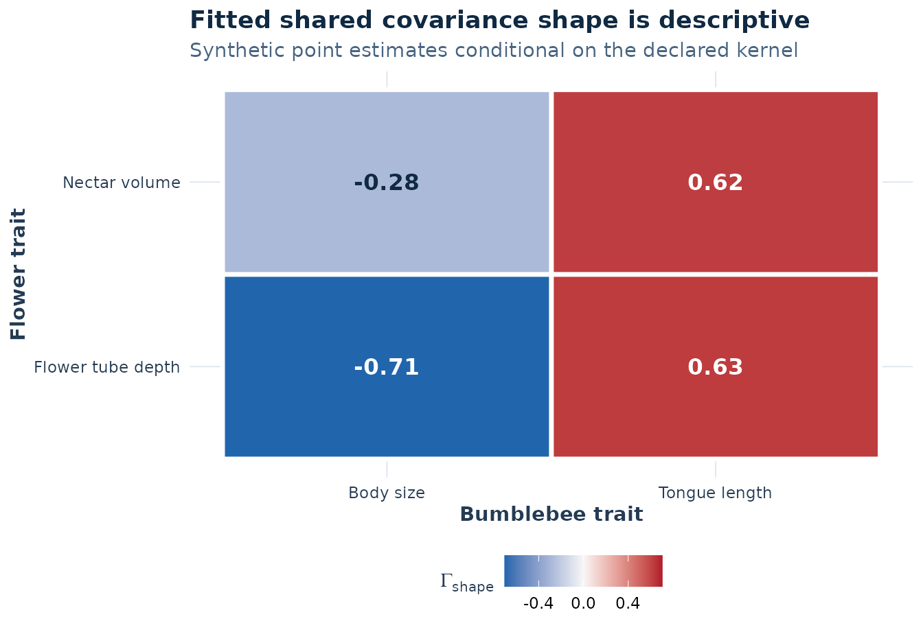

Fitted Gamma block for the synthetic example. Each tile is a point estimate of shared covariance shape between a flower trait and a bumblebee trait, conditional on the fixed kernel; no interval is shown because this workflow has no calibrated Gamma uncertainty.

Example 3: sensitivity to a small set of fixed bridge strengths

The bridge strength rho is a modelling choice in this workflow. A useful check is to refit a short grid of values chosen before looking at the fitted Gamma block. The curve below compares model fits at four fixed values; it is not a confidence interval and does not estimate rho in the engine.

In this synthetic fixture, a zero bridge fits much worse, whereas the three positive bridge strengths are almost tied. This is the useful conclusion from the display: the data separate “no bridge” from “some positive bridge” here, but do not choose a precise positive value. That is exactly why the plot is a sensitivity display rather than fitted-rho inference.

refit_cross <- function(K, rho) {
  gllvmTMB(
    traits(flower_tube_depth, nectar_volume, tongue_length, body_size) ~ 1 +
      kernel_latent(species, K = K, d = 2, name = "cross"),
    data = example$data_wide,
    unit = "observation",
    cluster = "species",
    family = gaussian(),
    control = gllvmTMBcontrol(se = FALSE)
  )
}

rho_profile <- profile_cross_rho(
  example$A_plant,
  example$A_bumblebee,
  example$W,
  rho = c(0, 0.25, example$truth$rho, 0.8),
  refit = refit_cross
)
rho_profile
#>    rho     logLik relative_logLik delta_deviance is_best convergence pd_hessian
#> 1 0.00 -163.01291     -243.654939     487.309878   FALSE           0         NA
#> 2 0.25   78.43539       -2.206636       4.413272   FALSE           0         NA
#> 3 0.55   79.43296       -1.209063       2.418126   FALSE           0         NA
#> 4 0.80   80.64203        0.000000       0.000000    TRUE           0         NA
#>   status error
#> 1     ok  <NA>
#> 2     ok  <NA>
#> 3     ok  <NA>
#> 4     ok  <NA>

rho_ok <- subset(rho_profile, status == "ok")

ggplot(rho_ok, aes(rho, relative_logLik)) +
  geom_hline(yintercept = 0, colour = "#9FB3C8", linewidth = 0.45) +
  geom_vline(
    xintercept = example$truth$rho, linetype = "dashed",
    colour = "#D64545", linewidth = 0.65
  ) +
  geom_line(colour = "#1261A0", linewidth = 0.8) +
  geom_point(colour = "#1261A0", fill = "white", shape = 21, size = 3,
    stroke = 0.9) +
  scale_x_continuous(breaks = rho_ok$rho, limits = c(0, 0.85)) +
  labs(
    title = "The data reject no bridge but do not identify one positive rho",
    subtitle = "The dashed rule marks the supplied teaching value; the positive plateau is nearly flat",
    x = expression("Fixed bridge strength " * rho),
    y = "Relative log likelihood (best fixed value = 0)",
    caption = "No confidence interval is implied: rho is rebuilt into the kernel for each refit."
  ) +
  theme_article()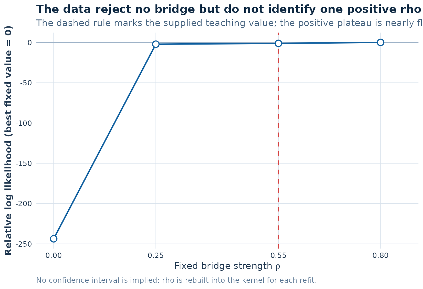

Fixed-rho sensitivity curve for the synthetic example. Relative log likelihood is shown only for four pre-specified, refitted kernels. The vertical rule marks the data-generating rho used for this teaching fixture; it is not an estimated parameter or confidence limit.

What to do with empirical data next

For an empirical analysis, first make the biological unit explicit: normally one row per measured organism or species-level replicate, with a documented link from each row to a tree tip. Then retain the four checks this small example makes visible: tree labels, trait availability, interaction-matrix ordering, and the smallest eigenvalue of the assembled kernel.

You can use profile_cross_rho() to refit a short, pre-specified grid of fixed rho values as a sensitivity analysis. The separate profile_cross_rho_ci() helper is screening-grade only: its fixed-grid coverage has not been calibrated, so do not present its output as a validated confidence interval. A bootstrap, a null calibration, or a broader model comparison is therefore a separate analysis plan, not a conclusion licensed by this article.