A conceptual integrated SDM case study for twelve species

Conceptual case study, not a copy-and-run tutorial. This page reports a retained simulation study and shows the modelling decisions it supports. Its analysis objects are not installed with the package, so copying every chunk into a fresh R session will not reproduce the reported numbers. For a self-contained workflow that simulates data, declares several observation sources, and fits the model from start to finish, use Integrating three data sources at once.

What this shows

You have two kinds of data on the same birds. One is opportunistic – eBird checklists, GBIF records – with counts, wildly uneven effort and no sampling design. (If those names are new: eBird is a global bird-recording platform built on checklists, and GBIF, the Global Biodiversity Information Facility, is the portal where species records from museums, surveys and citizen science are aggregated and downloaded.) The other is a structured survey: a protocol, fixed stations, detection or non-detection, and far fewer sites. An integrated species distribution model fits both at once.

The motivation, in one line, is that the designed sample should discipline the messy one – though note up front that this article does not test that: it never compares an opportunistic-only fit, a survey-only fit and the integrated one. What it does is run one integrated model end to end for twelve boreal songbirds, with the two sources at locations that share nothing at all, and finish with the thing the exercise is for: a map of relative intensity for all twelve species.

Twelve species rather than two, because twelve makes two decisions real that you will meet on your own data.

1. How many shared spatial gradients should the model fit? The species are tied together by unmeasured surfaces they all respond to, and you have to say how many. Decision 1: how many shared gradients? settles it with AIC, and shows why the rule of thumb most people reach for instead points one gradient too high.
2. What do you do about overdispersion? The count arm is Poisson, and Poisson has no dispersion parameter, so extra noise has to go somewhere. Decision 2: overdispersion in an arm with no dispersion parameter measures the option this package offers.

Getting the package. gllvmTMB is not on CRAN; install it from GitHub:

# install.packages("remotes")
remotes::install_github("itchyshin/gllvmTMB")
library(gllvmTMB)

Everything needed for your own data — isdm_sources(), make_mesh(), gllvmTMB(), and predict() — is in the installed package. The retained simulation objects used to calculate this page’s numerical results are not.

Two neighbouring questions have articles of their own rather than a paragraph here: how much survey you need (How big does an integrated survey design need to be?) and what repeat visits buy you (What do repeated survey visits add to an integrated model?).

The data are simulated

No real GBIF or ABMI (Alberta Biodiversity Monitoring Institute) data were analysed for this article. Everything below describes a simulated boreal songbird community shaped on a real system – Canada Warbler (Cardellina canadensis) and eleven co-occurring species in Alberta, an eBird-style opportunistic arm and an ABMI-style structured detection arm (a standardised provincial survey programme) – and no number here is a measurement about any real taxon.

Three reasons, all of which you would meet on the way to the real analysis:

1. The structured arm is not freely available at usable precision. ABMI publishes public survey locations fuzzed to roughly 5.5 km; precise coordinates need a separate data agreement, and fitting the fuzzed ones would measure the fuzz as much as the birds – the subject of the companion article When one data source knows where it is and the other does not.
2. A vignette must not depend on the network. rgbif will fetch the opportunistic arm, but a documentation build that phones an API is a documentation build that breaks.
3. Real integration needs cleaning and matching work that would swamp everything this page is trying to show.

Simulating also buys the one thing real data cannot: a known truth, against which did the model recover it is a question with an answer.

This simulation is the easy version of the problem, in two specific ways that matter for whether any of it transfers: the opportunistic records are scattered at random rather than clustered along roads, and the environmental covariate is uncorrelated with the unmeasured spatial structure by construction. Neither holds on real data. Before you use this on real data spells out what that leaves untested.

The two arms, and the one field they share

Everything here rests on a single idea: the two data sources are two ways of observing the same underlying abundance. Write the log of that abundance for species $j$ at location $i$ as

$$\eta_{ij} \;=\; \alpha_j \;+\; \beta_j\,\mathrm{env}_i \;+\; \lambda_{1j} f_{1i} \;+\; \lambda_{2j} f_{2i} \;+\; \log(\text{effort}_i) \;+\; \kappa\,\mathbf{1}\{\text{arm}_i = \text{opportunistic}\},$$

and read it one piece at a time.

$\alpha_j + \beta_j\,\mathrm{env}_i$ – the habitat part. Each species has its own intercept and its own slope on the environmental covariate, exactly as it would in a per-species GLM. These slopes are what most people came for.

$\lambda_{1j} f_{1i} + \lambda_{2j} f_{2i}$ – the shared unmeasured gradients. A latent spatial field is everything spatial you did not measure, estimated as a smooth surface: soil, moisture, disturbance history, whatever else organises the community. There are two of them here, estimated rather than supplied, and each species carries its own pair of loadings on them. A species with a large positive loading on the first surface is common where that surface runs high, and species with similar loadings co-occur – which is how a community model differs from twelve separate SDMs.

$\log(\text{effort}_i)$ – the offset. A known multiplier with no fitted coefficient: doubling the effort doubles the expected count, and the model is told that rather than asked to discover it. Any other known adjustment goes in the same place. If you carry QPAD-style detectability offsets for time of day, date and distance (Sólymos et al. 2013), add them into this term rather than modelling them separately.

$\kappa$ – the arm indicator. The two sources report on different overall scales, and one intercept per source absorbs that difference so the shared parts do not have to.

Counts and detections then come off that same $\eta$ by different routes: $y_{ij}\sim\text{Poisson}(e^{\eta_{ij}})$ on the opportunistic arm, and $y_{ij}\sim\text{Bernoulli}(1-e^{-e^{\eta_{ij}}})$ – a complementary log-log link – on the structured one. The cloglog link is not a taste: it is exactly the probability that a Poisson count with that same mean is at least one, so “at least one bird detected here” and “this many birds counted there” become statements about one abundance rather than two. isdm_sources() is what tells the model which rows follow which process.

The mesh, and why your two sources need not share a single site. A mesh is a triangulated grid laid over the study area. The latent field is estimated at the mesh nodes, and any location – from either arm – takes its value as a weighted average of the nodes around it. That is the whole mechanism by which two data sources sharing no row, no coordinate and no label share a field: the field lives on the mesh, not on the data.

That is the question that stops most people before they start. You do not need to match an eBird checklist to an ABMI station, grid both onto a common raster, or throw away the source with fewer sites. Build the mesh over the union of both, and project every row onto it.

The simulator draws the two arms independently over one landscape, so nothing here quietly assumes a convenience the real data will not have:

dat   <- sim_cawa12(seed = 1L)
truth <- attr(dat, "truth")
cells <- attr(dat, "cells")

str(dat[, c("cell_id", "trait", "isdm_source", "env", "log_effort", "value")])
#> 'data.frame':    4320 obs. of  6 variables:
#>  $ cell_id    : Factor w/ 360 levels "po001","po002",..: 1 2 3 4 5 6 7 8 9 10 ...
#>  $ trait      : Factor w/ 12 levels "CAWA","OVEN",..: 1 1 1 1 1 1 1 1 1 1 ...
#>  $ isdm_source: Factor w/ 2 levels "ebird","abmi": 1 1 1 1 1 1 1 1 1 1 ...
#>  $ env        : num  -1.294 1.426 -0.309 -1.223 1.372 ...
#>  $ log_effort : num  -1.0253 0.1086 0.4817 0.1118 -0.0946 ...
#>  $ value      : int  0 2 0 0 3 3 6 2 0 0 ...

This str() is the shape your own data has to reach, so read it as a target. One row per species per location. cell_id labels the location (give every location its own label — it is bookkeeping here, and the reference section shows it never enters the prediction). trait is the species. isdm_source says which dataset the row came from. value is the count on the opportunistic rows and detected/not-detected (1/0) on the survey rows. log_effort is the log of whatever measures how hard that row was looked for — checklist duration, point-count minutes — and any known detectability corrections you already compute (QPAD-style offsets for time of day, date, distance) are added into it. Building this frame from an eBird download plus your own survey table — stacking the two, agreeing on the covariate columns, constructing log_effort for each arm — is real work this page does not show; it is ordinary rbind() and dplyr work, but budget time for it.

What counts as a “site”? Whatever unit carries one location and one effort. In this simulation a site is a randomly placed point — despite the cell_id name, nothing here is a grid cell, and no gridding is required: the model works on exact coordinates, the spatial field is a continuous surface, and the mesh is a computational device for estimating it, not a grid your data must live on. In your own data an eBird checklist is a natural site (one place, one duration); pooling checklists into grid cells and summing their effort is a choice you may make, never a requirement. A survey station is a site as it stands. The whole question — sites, cells, checklists, and why the mesh is none of them — has its own short article: What is a site? The unit of analysis. And the table is a complete crossing: every site has a row for every species, zeros included. Those zeros are data — “we looked here and did not find this species” — and they exist in eBird only for complete checklists, where the observer reported everything detected. A raw presence-only download has no zeros to give, which is exactly why the presence-only section treats it as a different problem.

If your survey records counts rather than detections, keep them. Declare both arms Poisson — isdm_sources(ebird = poisson(), survey = poisson()) is accepted — and do not binarise your abundances.

tab <- table(cells$arm)
cat("opportunistic cells:", tab[["ebird"]],
    " structured stations:", tab[["abmi"]],
    "\nspecies:", length(truth$code), " rows:", nrow(dat), "\n")
#> opportunistic cells: 300  structured stations: 60 
#> species: 12  rows: 4320

## Disjoint by construction: no cell id, and no coordinate, is shared.
po <- cells[cells$arm == "ebird", ]; sv <- cells[cells$arm == "abmi", ]
cat("shared cell ids:", length(intersect(po$cell_id, sv$cell_id)),
    " shared (X, Y):",
    length(intersect(paste(po$X, po$Y), paste(sv$X, sv$Y))), "\n")
#> shared cell ids: 0  shared (X, Y): 0

## Effort varies WITHIN each arm, so the offset is not a relabelling of arm.
cat("sd(log effort) within arm:", f2(sd(po$log_effort), 3), "/",
    f2(sd(sv$log_effort), 3),
    " cor(log effort, arm):",
    f2(cor(cells$log_effort, cells$arm == "ebird"), 3), "\n")
#> sd(log effort) within arm: 0.685 / 0.364  cor(log effort, arm): -0.006

cat("largest opportunistic count:", max(dat$value[dat$isdm_source == "ebird"]),
    " detection rate, structured arm:",
    f2(mean(dat$value[dat$isdm_source == "abmi"]), 3), "\n")
#> largest opportunistic count: 49  detection rate, structured arm: 0.331

One thing to do before you mesh anything: project your coordinates. A degree of longitude and a degree of latitude are different physical distances everywhere but the equator, and a mesh built on degrees treats them as equal. These coordinates are in UTM kilometres inside a single zone. The projection comparison below returns to this, because the obvious way of checking such a choice – fit both and compare – does not work.

Fit it, and check that it is really a fit

t0 <- proc.time()[["elapsed"]]
f  <- cawa12_fit(dat)
elapsed <- proc.time()[["elapsed"]] - t0
fit <- f$fit

cat("model: "); print(cawa12_formula()[[3]])
#> model:
#> 0 + trait + trait:env + isdm_source + offset(log_effort) + spatial_latent(0 + 
#>     trait | coords, d = 2)
cat("\naccepted:", f$ok, " convergence:", f$convergence,
    " iterations:", f$iterations,
    "\nobjective:", f2(f$objective, 3), " seconds:", f2(elapsed, 1),
    " mesh nodes:", cawa12_mesh(dat)$mesh$n, "\n")
#> 
#> accepted: TRUE  convergence: 0  iterations: 136 
#> objective: 4949.806  seconds: 9.7  mesh nodes: 64

spatial_latent(0 + trait | coords, d = 2) is the shared field, with per-species loadings on it; d = 2 is the number of gradients, the subject of the next section. The mesh is built from dat – the union of both arms’ locations – and every row from either arm is projected onto it. The cutoff in make_mesh() – an interface inherited from sdmTMB, the single-species spatial package these helpers descend from – is the minimum spacing between mesh nodes, in the units of your coordinates – kilometres here, because the coordinates were projected first. This page uses cutoff = 40 on a domain roughly 225 by 443 km, giving 64 nodes: about a tenth of the domain’s shorter side is a reasonable starting point. A smaller cutoff means more nodes, a finer field, and a slower fit; if your conclusions change when you halve it, the mesh was too coarse.

This is a small example: 360 sampled locations, a 64-node mesh, about a minute per fit. Nothing on this page measures how any of it scales to tens of thousands of checklists or a mesh an order of magnitude larger.

convergence == 0 is not the check. This package can return convergence == 0 after a single iteration, at an astronomically large objective, with every spatial parameter still sitting at its starting value: a fit that never happened, reporting success. So look at iterations as well. Counts in the tens or hundreds are the healthy shape; 1 means the optimiser never moved. cawa12_fit() accepts a fit only when all three of convergence == 0, iterations > 1 and a finite objective hold.

Keep the counts moderate. That failure arrives when the counts get large, and large is not a feeling, so it was measured: the opportunistic arm’s overall intensity – the same $\kappa$ the model formula above carries as that arm’s intercept, here set in the simulation – was raised step by step, three datasets per step. kappa in the table below is the value it was set to.

#>   kappa mean_ct  max_ct   iters  ok        verdict
#> 1   1.0    1.76   34-40  98-167 3/3        healthy
#> 2   2.3    6.46 136-147 168-186 3/3        healthy
#> 3   2.4    7.17 142-157   13-14 0/3 no convergence
#> 4   3.0   12.96 268-272     1-1 0/3    1 iteration

Two things to take from that. The cliff is not far off – fits are healthy up to a mean cell count near 6.5 and all three seeds fail one step later – and a cap on the largest single cell is a poor early-warning sign, because the largest count overlaps across the cliff (147 in a healthy fit against 142 in a rejected one); what controls it is the mean cell intensity. So keep your largest cell count under about 100 is a recommendation with margin, not a measured threshold.

Accuracy starts decaying two steps before the optimiser breaks, while every fit still reports itself healthy. The full sweep, and the recovery numbers behind that sentence, are in the full count-ceiling sweep.

What this one fit recovered

est <- cawa12_env_slopes(fit)
cmp <- data.frame(species = truth$code, truth = round(truth$beta, 3),
                  estimate = round(unname(est), 3))
cmp$error <- round(cmp$estimate - cmp$truth, 3)
cmp
#>    species  truth estimate  error
#> 1     CAWA  1.280    1.243 -0.037
#> 2     OVEN  0.549    0.733  0.184
#> 3     TEWA -0.182   -0.004  0.178
#> 4     BLPW  1.156    0.895 -0.261
#> 5     BBWA  0.538    0.473 -0.065
#> 6     BTNW  0.855    1.061  0.206
#> 7     CMWA  0.425    0.062 -0.363
#> 8     MAWA -0.054   -0.340 -0.286
#> 9     SWTH  0.028   -0.040 -0.068
#> 10    WTSP -0.174   -0.448 -0.274
#> 11    YRWA  1.028    0.619 -0.409
#> 12    RBNU  0.524    0.610  0.086
cat("cor(estimate, truth):", f2(cor(cmp$estimate, cmp$truth), 3),
    " mean |error|:", f2(mean(abs(cmp$error)), 3),
    " mean signed error:", f2(mean(cmp$error), 3), "\n")
#> cor(estimate, truth): 0.915  mean |error|: 0.201  mean signed error: -0.092

That is one dataset, and a single replicate scatters. Read it against the 12-seed envelope instead: correlation with truth 0.936, sd 0.026. Judging an estimator from one replicate is how people conclude it is broken when it is not.

The slopes do come back shrunk, here and in every replicate: the mean signed error across the campaign is -0.149 against a true slope SD of 0.514. This article makes no claim that these estimates are unbiased.

Decision 1: how many shared gradients?

Verdict: fit d = 1, 2, 3, 4, and take the lowest AIC. On ten replicate datasets whose true number of gradients is 2, AIC picked 2 in 10 of 10. The rule of thumb you would otherwise reach for – fit a generous number, then stop where a loading column goes near zero – got it right in 1 of 10, and no threshold rescues it.

d is the number of independent unmeasured gradients the community responds to. d = 1 says one hidden surface organises all twelve species; d = 4 says four do. The model will fit whichever number you write, without complaint, which is why this is a decision and not a setting.

#>   d df mean_AIC        AIC_range median_secs mean_delta_AIC
#> 1 1 38  10055.4 9894.5 - 10195.3        26.0         140.36
#> 2 2 49   9915.0 9733.2 - 10043.1        53.4           0.00
#> 3 3 59   9932.9 9753.2 - 10062.7        80.1          17.85
#> 4 4 68   9950.8 9771.2 - 10080.7       129.9          35.81
#> AIC picks d = 2 in 10 of 10 replicates; BIC picks d = 2 in 10

Fitting too few gradients is expensive – d = 1 costs 81.2 units of log-likelihood on average – while each gradient past the truth buys almost nothing and pays about 20 AIC for the privilege. That asymmetry is why AIC lands on the right answer so consistently here. One caveat on the comparison itself: at a superfluous rank (a number of gradients d above the truth) the extra loading column sits on the boundary of its parameter space, so AIC’s nominal penalty is conservative in the direction that flatters all ten results – the same boundary problem noted for Psi in the overdispersion study.

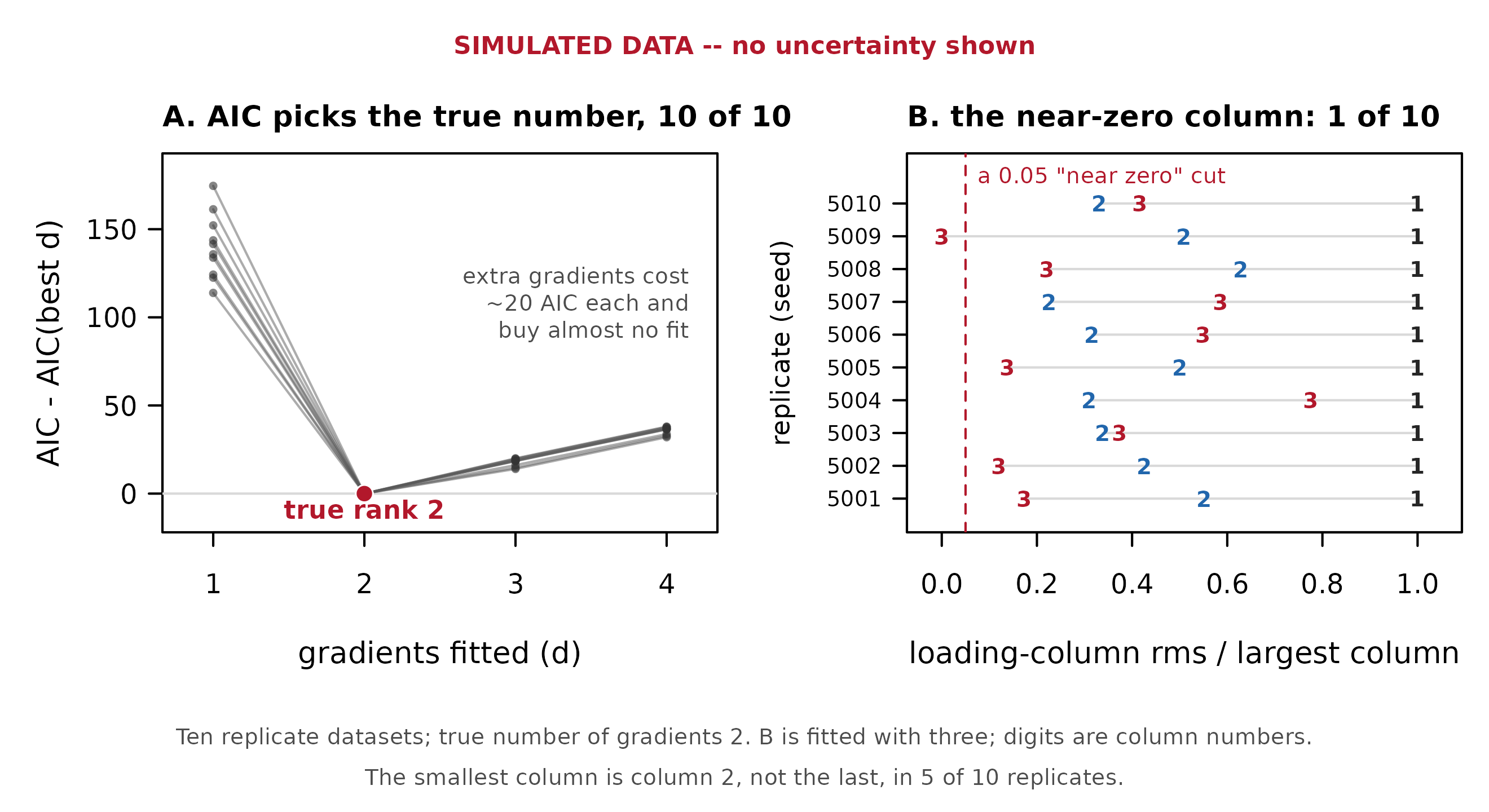
Choosing the number of shared gradients on ten replicate datasets whose true number is 2. Panel A plots each replicate’s AIC relative to its own best value: the minimum falls at d = 2 in every replicate, fitting too few at d = 1 costs 114 to 175 AIC units, and each gradient beyond the truth costs about 20 AIC for almost no gain in fit. Panel B tests the rule of thumb AIC is competing against. Each replicate was fitted with one gradient too many, and the three loading columns’ root-mean-square values are plotted relative to the largest, the digit giving the column number. A reader stopping when a column falls below a near-zero cut reads the answer correctly in one replicate of ten: the smallest of the three columns runs from 0.00 to 0.34 of the largest, with only one replicate below a 0.05 cut, and the SMALLEST column is column 2 rather than the last in five of the ten replicates, because the fitted columns get mixed among themselves. No uncertainty is shown anywhere in this figure.

Why the near-zero-loading rule fails

It fails for a reason worth knowing, because it is not specific to this package. The fitted loading columns are not pinned to particular gradients: any rotation of them describes the same model equally well, so the columns come out mixed among themselves. “The extra column” is therefore not the last column. Fitted with three gradients, the smallest column is column 2 rather than column 3 in 5 of 10 replicates. A reader following the recipe inspects the third column, finds a substantial value, and concludes the third gradient is real. Panel B above is that fact drawn.

Even ignoring the ordering, the gap is not there to find: an unneeded direction does not always collapse to zero, and nothing inside a single fit separates “a tenth of the leading gradient” from a weak real one. So compare by AIC. If you want a loading-based sanity check anyway, use the singular values of the loading matrix rather than its columns – they are at least immune to the mixing – quote your threshold, and treat the answer as a hint. Here is that matrix for the live fit:

L <- fit$report$Lambda_spde          # 12 x d -- use this, not the packed vector
dim(L)
#> [1] 12  2
round(sqrt(colMeans(L^2)), 4)        # per-column rms
#> [1] 0.0352 0.0196
round(svd(L)$d / max(svd(L)$d), 4)   # singular values, relative to the largest
#> [1] 1.0000 0.5321

Use fit$report$Lambda_spde rather than the packed parameter vector: the packed version holds P*d - d*(d - 1)/2 values rather than P by d, so naming it with your species vector mislabels silently.

What it costs

#>   d median_secs_per_fit fits_in_this_campaign
#> 1 1                26.0                    10
#> 2 2                53.4                    10
#> 3 3                80.1                    10
#> 4 4               129.9                    10

Fitting four values of d on one dataset is a few minutes at this size. You do not have to repeat the ten-dataset campaign – fit your own d = 1..4 once and read the AIC.

Decision 2: overdispersion in an arm with no dispersion parameter

Verdict. In this simulation, spatial_latent(..., unique = TRUE) substantially improved the point estimates – RMSE in the environmental slopes fell from 0.305 to 0.177 – but by a mechanism that looks more like regularisation than like estimating the overdispersion: how far a slope moved tracked the base model’s own error (-0.88) far more closely than it tracked the species’ simulated overdispersion (0.36). Do not read Psi as a measurement of how overdispersed your counts are, and do not expect your intervals to improve. It costs about 2.8 times the runtime and makes fits less stable. And you cannot tell from a variance-to-mean ratio whether you need it.

Here is the problem in terms you already have. With an overdispersed Poisson GLMM you would add an observation-level random effect and let it soak up the extra noise. This model has no such tier by default, so extra-Poisson variation goes to the term with the most freedom to absorb it: the shared spatial field. A field busy mopping up observation noise is not estimating space, and your slopes are estimated conditionally on it – which is how overdispersion you ignored comes back as bias in the slopes you care about.

spatial_latent(..., unique = TRUE) adds a per-species tier of its own, called Psi, alongside the shared field, to play a role similar to the observation-level random effect in a GLMM – similar, not identical: Psi is itself spatially structured rather than independent noise per row, which is part of why its behaviour below is odd, and the record section says more. It has to be asked for:

value ~ 0 + trait + trait:env + isdm_source + offset(log_effort) +
  spatial_latent(0 + trait | coords, d = 2, unique = TRUE)

It was measured rather than argued: overdispersion was added to the opportunistic arm only, the twelve species carrying a ladder of severity from 0.00 (none at all) to 0.90, and both models were fitted to identical data on an identical mesh.

Your counts will look overdispersed even when they are not

The obvious pre-fit check is the variance-to-mean ratio, and it misleads. The table puts the observed VMR beside a matched counterfactual – same landscape, same effort, same species, simulated with no overdispersion at all.

#>    species sigma   VMR VMR_no_overdisp frac_above
#> 1     CAWA  0.00  7.34            7.70       0.42
#> 2     MAWA  0.10  7.41            7.22       0.58
#> 3     OVEN  0.15  3.65            3.51       0.58
#> 4     RBNU  0.20  2.70            2.58       0.62
#> 5     TEWA  0.30  2.11            1.89       0.73
#> 6     SWTH  0.35  2.00            1.76       0.73
#> 7     BLPW  0.45  9.13            7.55       0.73
#> 8     WTSP  0.55  8.30            6.91       0.65
#> 9     BBWA  0.60  4.23            3.09       0.92
#> 10    YRWA  0.70  7.46            4.73       0.85
#> 11    BTNW  0.75 10.08            5.41       1.00
#> 12    CMWA  0.90  8.65            3.97       1.00

That counterfactual column runs from 1.8 to 7.7 with no overdispersion at all: the shared spatial field, the environmental gradient and the varying effort inflate it on their own. So “VMR far above 1” does not demonstrate overdispersion in a model like this one – and on real data you have no counterfactual to compare it against. Only at the top of the ladder is the contrast clear; at $\sigma \le 0.45$ the observed VMR beats its own counterfactual in 0.42 to 0.73 of replicates, which is a coin flip dressed up as a diagnostic.

What turning it on actually did

#>                                                 quantity  value
#> 1              median |change| in env slope, in base SEs  0.429
#> 2                         median SE ratio, unique / base  0.821
#> 3   95% coverage of the true slope (est ± 1.96 SE), base  0.869
#> 4 95% coverage of the true slope (est ± 1.96 SE), unique  0.982
#> 5                                             bias, base -0.183
#> 6                                           bias, unique -0.110
#> 7                                             RMSE, base  0.305
#> 8                                           RMSE, unique  0.177

The expected story is that ignoring overdispersion makes your intervals too narrow and the fix widens them. That is the wrong way round here. The slopes move – about 0.43 of a standard error at the median – and the standard errors move down, not up (median ratio 0.821). The plausible reading is that the base model’s coverage failure was bias rather than understated uncertainty: freeing the shared field from having to absorb observation noise de-attenuates the slopes and tightens them at once. Take that as the likely direction rather than a settled result – the coverage figures come from 22 replicate pairs, twelve species inside each sharing one estimated field, and carry no uncertainty of their own. Coverage rises from 0.869 to 0.982, overshooting the nominal 0.95, so this is no route to well-calibrated intervals either.

Psi itself is a threshold detector, not a measurement: below about $\sigma = 0.5$ it sits at zero, and above it, it fires in most replicates but recovers only 1 to 21 per cent of the true variance.

And it costs stability. The unique model failed to produce a usable curvature matrix – the thing standard errors are computed from – in 5 of the 14 pairs where both models returned standard errors. Variance components pinned at zero are where that happens.

#> over 22 pairs -- median delta logLik (unique - base): 12.58 
#> extra parameters: 12  median delta AIC: 1.15 
#> replicates favouring unique: 11 of 22

By likelihood it fits clearly better; by AIC it barely pays, and only in about half the replicates. Restricting the comparison to the pairs with a well-behaved curvature matrix reproduces every number above, so none of it is an artefact of that subset – details, and one caveat about testing the log-likelihood difference, in the overdispersion study.

The map

Three things have to be right before a surface means anything.

The spatial field must be in the prediction. The current gllvmTMB 0.7.1 source contains the ordinary SPDE prediction repair. Early 0.7.0 source snapshots did not all contain it; this saved map was reproduced from a source snapshot that included the repair. A version string alone is therefore not enough to identify the code used for an older saved map. Before trusting an older saved map, reproduce the training-row identity predict(fit, newdata = training_rows) == predict(fit). The current public route covers the ordinary intercept-only SPDE point predictor, not spatial slopes.

The scale must be effort-free. type = "response" includes the row’s offset, so it returns an expected count at that effort – right for a training row, wrong for a map. Setting log_effort to zero on the grid gives relative intensity, exactly rather than approximately, because the offset is re-evaluated against newdata.

The covariate must be on the scale it was fitted on. env was standardised once, on the training data, and the grid must reuse those same two numbers. Re-standardise the grid on its own mean and SD and the map’s pattern survives almost untouched while its values do not – so no visual check will catch it.

grid <- md$grid[, c("X", "Y", "env")]     # already on the TRAINING scale
newd <- do.call(rbind, lapply(levels(dat$trait), function(sp)
  transform(grid, trait = sp)))
newd$trait       <- factor(newd$trait, levels = levels(dat$trait))
newd$cell_id     <- factor("po001", levels = levels(dat$cell_id))
newd$isdm_source <- factor("ebird", levels = levels(dat$isdm_source))
newd$log_effort  <- 0                     # relative intensity, NOT a count

p <- suppressWarnings(suppressMessages(
  predict(fit, newdata = newd, type = "response")))
E <- matrix(p$est, ncol = nlevels(dat$trait),
            dimnames = list(NULL, levels(dat$trait)))
cat("grid cells:", nrow(grid), " species:", ncol(E),
    " relative intensity:", f2(min(E), 3), "to", f2(max(E), 2), "\n")
#> grid cells: 1326  species: 12  relative intensity: 0.018 to 17.33

## The saved surfaces the figure is drawn from came from this same fit.
agree <- max(abs(E - md$est))
cat("max |live prediction - saved surface|:", signif(agree, 3), "\n")
#> max |live prediction - saved surface|: 0.00022

The figure below is drawn from those saved surfaces. The line above is the check that the fit you have just run reproduces them: the largest disagreement anywhere on the grid is 2.2^{-4}, against surface values running from 0.018 to 17.33.

newd deliberately has no response column. A prediction grid describes the locations and covariates at which to evaluate the fitted model; current predict() builds its design from the right-hand side and does not require a dummy outcome.

What the map does not carry – read this before the picture

No uncertainty, of any kind. There is no interval behind any value in the figure below. se.fit is refused outright with newdata, and the refusal is deliberate rather than an oversight:

cat(err_of(predict(fit, newdata = newd, type = "link", se.fit = TRUE)))
#> <gllvmTMB_predict_se_newdata_unsupported>
#> `se.fit = TRUE` is not yet supported together with `newdata`.
#> ℹ Standard errors are currently only available for the training rows (`newdata
#>   = NULL`).

The standard error that is available at training rows ignores the error in reconstructing the latent field, which is exactly what dominates on a map. Map-scale uncertainty needs random-effect-aware machinery that is not calibrated here. In a retained 1,600-fit negative control, the fixed-only standard error covered the true linear predictor only 0.23–0.82 of the time. That is why the refusal remains. A separate 22,200-fit campaign for a fixed trait:env coefficient met its prespecified narrow coverage criterion, but fixed-coefficient coverage does not transfer to a reconstructed spatial surface.

Prediction accuracy at withheld locations has not been established. Training-row identity proves that the fitted field is reconstructed and packed correctly; it does not show how accurately the model predicts withheld locations.

Nothing outside the mesh. The grid deliberately extends 6 per cent beyond the sampled extent, the way a real prediction map would, and predict() says so:

cat(warn_of(suppressMessages(predict(fit, newdata = newd, type = "response"))))
#> <gllvmTMB_predict_newdata_outside_mesh>
#> 288 `newdata` rows fall outside the mesh hull.
#> ✖ The spatial field is exactly 0 there -- not estimated, and not
#>   distinguishable from a field that is genuinely near zero.
#> ℹ Restrict `newdata` to the meshed domain, or rebuild the mesh to cover it.

Out there the mesh basis is all zeros, so the field is exactly zero – indistinguishable, on a coloured surface, from a region where the field is genuinely near zero. A blank corner reads as a cold one. 24 of 1326 cells are in that state here, and the figure hatches them rather than colouring them. Clip your grid, or extend your mesh; do not suppress the warning, which is what the chunk above did purely to keep the figure inline.

A little extrapolation in the covariate. 58 of 1326 grid cells carry an env value outside the training range, a consequence of that same padding.

No claim that the slopes behind it are unbiased. They come back shrunk, as the recovery table above showed.

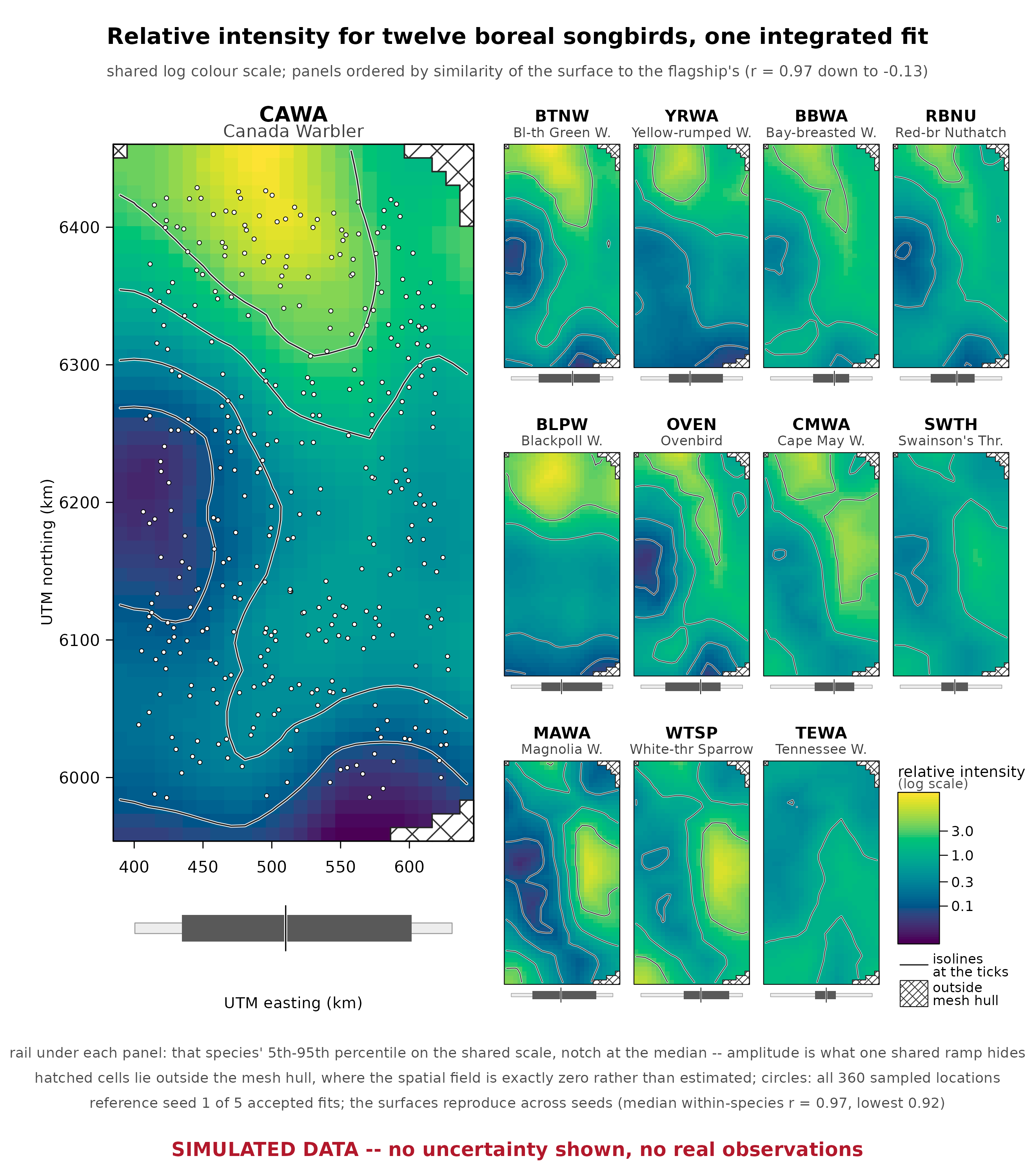
Relative intensity for all twelve species from one integrated fit, on a shared logarithmic colour scale. Canada Warbler is drawn large, carrying the axes in projected UTM kilometres, the sampled locations and the labelled scale; the other eleven are thumbnails ordered by the correlation of each surface with the flagship’s, so the grid reads as a gradient from most like it to opposite rather than as an arbitrary sequence. Colour is never the only channel: isolines at the same levels as the colour-bar ticks are drawn on every panel, and the rail under each panel places that species’ 5th to 95th percentile and median on the shared scale, because a shared ramp is exactly what compresses amplitude away. Cells outside the mesh hull are hatched rather than coloured: there the spatial field is exactly zero because the mesh basis is empty, not because it was estimated to be small. The surfaces carry NO uncertainty of any kind. The simulated-data fence is drawn inside the canvas because a PNG lifted into a talk keeps its pixels and loses its caption.

The map is drawn from one dataset. Across 5 replicates on the same landscape the drawn quantity replicates well – median within-species correlation of the log surfaces 0.974, lowest single pairing 0.916. That is a statement about the surface’s stability, not about its uncertainty.

If your opportunistic arm has no counts

eBird checklists carry counts. Many opportunistic downloads do not: a raw GBIF export is often presence-only – a location, a species, and nothing to put in value.

The standard route (Warton & Shepherd 2010; Renner et al. 2015) is to fit an inhomogeneous Poisson process as a weighted Poisson GLM: each presence record becomes a row with a tiny weight w and response y = 1/w, and a grid of background quadrature nodes covering the study area becomes rows with weight equal to their cell area and response y = 0. Fitted that way, the GLM’s likelihood is the point-process likelihood. gllvmTMB() accepts exactly that through weights =:

po <- rbind(
  data.frame(trait = sp, env = env_at_presences, y = 1e6, w = 1e-6),
  data.frame(trait = sp, env = env_at_nodes,     y = 0,   w = cell_area)
)
gllvmTMB(y ~ 0 + trait + trait:env, data = po, trait = "trait",
         unit = "obs_id", family = poisson(), weights = po$w)

The device recovers the true environmental slopes in this setting: over 12 species and 20 replicate datasets no species differed detectably from its true value, and a pooled test for uniform attenuation gave 1.0016 against a true value of 1. What that test could and could not have detected, and how dense the quadrature grid needs to be, are in the presence-only simulation results.

The package warns about such a fit, in its own words:

Non-unit likelihood weights create a weighted objective, not an ordinary
maximum-likelihood fit.
ℹ Point estimates remain available, but ordinary Hessian/Wald uncertainty,
  logLik(), AIC(), BIC(), and likelihood-ratio interpretations are not
  validated for this fit.
→ Use unit weights for likelihood-based inference. A sandwich-variance route
  has not yet been certified.

It does not combine with the two-arm model. Passing weights into an isdm_sources() fit is refused:

`weights` is not admitted for the integrated multi-source model.
✖ Across this model's arms `weights` would mean two different things: a
  binomial trial count on the detection rows and a likelihood multiplier on the
  count rows.
ℹ Repeated survey visits belong in the data as separate detection/non-detection
  rows, each carrying its own support in the `offset()`.
→ Drop `weights` and give each visit its own row.

If your opportunistic arm is genuinely presence-only, fit it with the quadrature device on its own, the way the standalone Joint ecological intensity from opportunistic records article does.

Do you need grid cells? No — and here is what they would cost

Nothing on this page was gridded. Every observation sits at its exact coordinates, the spatial field is a continuous surface, and the mesh is the computer’s scaffolding for that surface, not a grid the data live on. What a “site” is, why a count needs an observation event rather than a map square, and why the mesh is not a grid are untangled properly in What is a site? The unit of analysis.

But gridding is what many workflows are used to, so the cost of doing it anyway was measured rather than argued: the same twelve-species datasets were refitted with every location snapped to the centre of its grid cell and the habitat value re-read there — which is what gridding does to your data. Six datasets per cell size:

data.frame(cell = c("exact points", "6 x 11 km", "12 x 22 km", "25 x 44 km"),
           mean_cor = gr$cor.1, sd_cor = gr$cor.2,
           mean_abs_err = gr$mae.1, sd = gr$mae.2)
#>           cell mean_cor sd_cor mean_abs_err    sd
#> 1 exact points    0.926  0.036        0.244 0.068
#> 2    6 x 11 km    0.943  0.031        0.245 0.042
#> 3   12 x 22 km    0.946  0.027        0.257 0.065
#> 4   25 x 44 km    0.912  0.041        0.385 0.067

Two things to read off it.

Cells of typical atlas sizes cost nothing here. At 6 × 11 km and even 12 × 22 km, slope recovery is indistinguishable from exact coordinates.

The damage starts when displacement approaches the habitat’s own scale — and it looks like shrinkage, not scrambling. At 25 × 44 km cells a record can move ~25 km from where it was, the typical slope error rises from 0.244 to 0.385 — about 58% worse — while the species ranking barely moves (correlation 0.912). Gridding too coarsely does not make your results look wrong; it quietly pulls the habitat effects toward zero. That is the same positional-error mechanism the companion article When one data source knows where it is and the other does not measures in depth, and the same number decides it: displacement relative to the distance over which your habitat layer changes. This landscape’s habitat changes over ~100 km, so small cells are harmless; on a patchy 10-km-scale habitat layer the free zone would shrink accordingly — compute the ratio for your own raster with that article’s recipe rather than reusing these cell sizes.

One honest limit: this measured only the positional cost of gridding — the records moved, but each site kept its own row. Pooling many checklists into one cell row (summing counts and effort) changes the data in additional ways not measured here. And the choice of cell size is a genuine model choice: analyses of the same data on different grids can disagree with each other, which is a documented problem in spatial statistics, not a rounding curiosity.

Before you use this on real data

This simulation lives in the friendly regime, and that is the biggest caveat on the page. Two things are true here by construction and are false almost everywhere else. First, the latent surfaces are residualised against env, so the environmental covariate and the unmeasured spatial structure are uncorrelated; on real data habitat and unmeasured spatial structure are correlated in essentially every dataset, and the price of getting that wrong is not small – in this same simulator, removing the residualisation drives the estimated slopes to about +21 against a true mean near +1.3. How the model behaves under realistic covariate-field correlation is measured nowhere on this page, and it is the first thing to establish before trusting a slope from real data. Second, the opportunistic arm’s bias is a single constant, so its sampling is spatially uniform: preferential sampling – birders on roads, near towns and trailheads – is untested here, and it is the failure mode this literature worries about most.

Nothing here shows that integrating helped. This page never fits the opportunistic arm alone, the survey alone, and the two together and compares them. That comparison is the standard one in this field, and it is the obvious next thing to run on your own data.

The slopes come back shrunk. Every recovery table on this page shows a consistent downward pull. Do not describe estimates from this machinery as unbiased, and do not build an effect-size claim on their magnitude without running your own recovery check.

The map carries no uncertainty at all. Not a confidence interval, not a standard error, not a coefficient of variation. A smooth colourful surface implies precision it does not have, and this one has none to report.

Your survey coordinates are probably fuzzed, and that matters. Real structured-survey data frequently does not know exactly where it is – public ABMI locations are displaced by kilometres – and the consequences are not small. Read When one data source knows where it is and the other does not before fusing real fuzzed data. In particular, do not expect coarsening your raster to fix it: Gábor et al. (2022) is the direct test of that intuition, and the intuition does not survive it.

The specific numbers are properties of this design. AIC’s 10 of 10, the loading rule’s 1 of 10, the overdispersion results: all measured at twelve species, one landscape, one true number of gradients, moderate counts, and a small mesh. The mechanisms generalise; the hit rates do not.

Recap

isdm_sources() names the two observation processes. The arms sit at disjoint locations and still share one field, because the field lives on a mesh built over the union of both and every row is projected onto it. Project your coordinates before meshing. Check iterations, not just convergence, and keep your counts well under the ceiling. Choose the number of shared gradients by AIC, not by hunting for a small loading column. Consider unique = TRUE when a count arm may be overdispersed – in this simulation it clearly helped the point estimates, by a mechanism that looks more like regularisation than like estimating the overdispersion, so do not read Psi as a measurement and do not expect your intervals to improve. Zero the offset on the prediction grid, keep the covariate on its training scale, and hatch whatever falls outside the mesh.

Point estimates and a surface. No intervals – and this page says so, rather than letting a smooth picture imply otherwise.

A first-time reader can stop here. What follows is reference material: four behaviours to know about on the day something does not work, followed by details of the simulation evidence behind the numerical results.

Reference: four things that do not do what you would guess

Each of these is an algebraic identity, not a tendency measured on a sample: it holds exactly, for the reason given, and no number of replicates would make it more or less true. They are collected here because each has cost somebody an afternoon.

They are demonstrated on a deliberately small model – three of the twelve species – because the size of a fit cannot change an identity.

sub <- droplevels(dat[dat$trait %in% c("CAWA", "OVEN", "TEWA"), ])
fam <- isdm_sources(ebird = poisson(), abmi = binomial(link = "cloglog"))
msh <- make_mesh(sub, c("X", "Y"), cutoff = 40)
FIT <- function(f, ...) suppressMessages(suppressWarnings(gllvmTMB(
  f, data = sub, trait = "trait", unit = "cell_id", family = fam,
  silent = TRUE, ...)))

1. An offset that never varies within an arm does nothing

An offset() is a known multiplier with no estimated coefficient – data, not a parameter – so it cannot compete with anything for fit. If it never varies within an arm, the arm’s own intercept reproduces it exactly, and adding it changes nothing:

sub$const_off <- ifelse(sub$isdm_source == "ebird", 1.0, 0)   # constant per arm
o_none  <- FIT(value ~ 0 + trait + trait:env + isdm_source)$opt$objective
o_const <- FIT(value ~ 0 + trait + trait:env + isdm_source +
                 offset(const_off))$opt$objective
o_vary  <- FIT(value ~ 0 + trait + trait:env + isdm_source +
                 offset(log_effort))$opt$objective
c(no_offset = o_none, constant_offset = o_const, varying_offset = o_vary)
#>       no_offset constant_offset  varying_offset 
#>        1627.930        1627.930        1376.184
cat("relative difference, constant offset vs none:",
    format((o_const - o_none) / o_none, digits = 3), "\n")
#> relative difference, constant offset vs none: -1.6e-11

The first two are the same model to well inside the optimiser’s own tolerance. The real log_effort offset varies within each arm, which is why removing it does change the objective. If your own effort is one number per source, your offset is a relabelling of your source indicator, and the offset idiom is not doing anything for you.

2. The unit column of a prediction grid, and when it stops being inert

The design matrix requires some valid factor level in the unit column. In this model the only random effect is the spatial field, keyed on (X, Y), so the choice is arbitrary – provably so:

alt <- newd; alt$cell_id <- factor("sv060", levels = levels(dat$cell_id))
p_alt <- suppressWarnings(suppressMessages(
  predict(fit, newdata = alt, type = "response")))
cat("max |difference| between the two unit levels:",
    max(abs(p$est - p_alt$est)),
    "\nover a prediction range of", f2(diff(range(p$est)), 2), "\n")
#> max |difference| between the two unit levels: 0 
#> over a prediction range of 17.32

Exactly zero – an opportunistic cell’s label and a survey station’s give the same answer. This stops being true the moment your model has a genuine unit-level random effect. Then the label you wrote on the grid is used: predict() re-adds the matching random effect and tells you it has done so.

set.seed(3)
n <- 150; ev <- rnorm(n); site_eff <- rnorm(n, 0, 0.8)
toy <- do.call(rbind, lapply(1:2, function(j) data.frame(
  site = factor(seq_len(n)), env = ev, trait = c("a", "b")[j],
  value = rpois(n, exp(0.5 + c(0.9, -0.4)[j] * ev + site_eff)))))
toy$trait <- factor(toy$trait)
toy_fit <- suppressWarnings(suppressMessages(gllvmTMB(
  value ~ 0 + trait + trait:env + (1 | site), data = toy, trait = "trait",
  unit = "site", family = poisson(), silent = TRUE)))
toy_grid <- expand.grid(env = seq(-2, 2, length.out = 10),
                        trait = levels(toy$trait))
toy_grid$value <- 0
g1 <- transform(toy_grid, site = factor("1",  levels = levels(toy$site)))
g2 <- transform(toy_grid, site = factor("77", levels = levels(toy$site)))
cat(msg_of(predict(toy_fit, newdata = g1, type = "link")))
#> ℹ Random effects re-added on `newdata` for: "re_int" (where site / species
#>   levels matched the training factors).

q1 <- suppressMessages(predict(toy_fit, newdata = g1, type = "link"))
q2 <- suppressMessages(predict(toy_fit, newdata = g2, type = "link"))
cat("\nsite \"1\" vs site \"77\":", f2(max(abs(q1$est - q2$est)), 3),
    "on the link scale\n")
#> 
#> site "1" vs site "77": 0.447 on the link scale

So pick that level deliberately, or ask for a prediction with no site effect in it at all using re_form = ~0. Neither is what this article’s map uses, and on purpose: re_form = ~0 would zero the spatial field too, and that field is the entire point of the map.

3. The name after the | in a spatial term is ignored

There is no column called coords in the data, and there does not need to be. The geometry comes entirely from mesh =; the token to the right of the | is never read.

sp_obj <- function(tok) FIT(stats::as.formula(paste0(
  "value ~ 0 + trait + trait:env + isdm_source + offset(log_effort) + ",
  "spatial_latent(0 + trait | ", tok, ", d = 1)")), mesh = msh)$opt$objective
o <- c(coords = sp_obj("coords"), banana = sp_obj("banana"),
       cell_id = sp_obj("cell_id"))
o
#>   coords   banana  cell_id 
#> 1215.772 1215.772 1215.772
cat("largest difference:", max(o) - min(o), "\n")
#> largest difference: 0

cell_id is a real column with a real meaning, and it makes no difference whatsoever – which is the direction that matters. Writing spatial_latent(0 + trait | site) with a real site column and a real intention will also be ignored, and nothing will say so.

4. A mesh passed without a spatial term does nothing

mesh = is consumed by the spatial_*() term and by nothing else. With no such term in the formula, a mesh built with make_mesh() changes nothing – the fit runs, converges, and is entirely non-spatial:

m <- c(no_mesh   = FIT(value ~ 0 + trait + trait:env + isdm_source +
                         offset(log_effort))$opt$objective,
       with_mesh = FIT(value ~ 0 + trait + trait:env + isdm_source +
                         offset(log_effort), mesh = msh)$opt$objective)
m
#>   no_mesh with_mesh 
#>  1376.184  1376.184
cat("difference:", abs(diff(m)), "\n")
#> difference: 0

The package now warns for this case. Whether the warning reaches you depends on the path – when this page was built, the integrated fit above produced no warning:

cat(warn_of(gllvmTMB(
  value ~ 0 + trait + trait:env + isdm_source + offset(log_effort),
  data = sub, trait = "trait", unit = "cell_id", family = fam,
  silent = TRUE, mesh = msh)))
#> <gllvmTMB_unused_mesh>
#> ! `mesh` was supplied but the formula has no spatial term, so the mesh is
#>   unused.
#> ℹ Either add a `spatial_indep()`/`spatial_scalar()`/`spatial_latent()` term, or
#>   drop `mesh` if it was left over from a term that was removed.

So check that the spatial_*() term is in your formula rather than trusting a complaint to arrive. The objectives above are the reliable evidence: identical to the last decimal means the mesh did nothing.

The other raw-mesh case is loud and correct – a raw fm_mesh_2d() object with a spatial term is refused, which matters because most fmesher and INLA tutorials teach you to build one by hand:

raw_bnd  <- fmesher::fm_extensions(cbind(sub$X, sub$Y), convex = c(30, 60))
raw_mesh <- fmesher::fm_mesh_2d(loc = cbind(sub$X, sub$Y), boundary = raw_bnd,
                                max.edge = c(40, 120))

cat(err_of(FIT(value ~ 0 + trait + trait:env + isdm_source + offset(log_effort) +
                 spatial_latent(0 + trait | coords, d = 1), mesh = raw_mesh)))
#> <rlang_error>
#> Pass `mesh` as a result of `make_mesh()`.

Evidence behind the results

This section describes the simulation studies behind the numbers above, the measurements that did not make the main path, and the places where the evidence is weaker than a plain sentence would suggest.

Where the numbers come from

One fit runs live on this page. Everything replicated is read from a saved campaign:

#>                                campaign fits                           evidence
#> 1 intensity ceiling + recovery envelope   95 count-ceiling and recovery results
#> 2                        rank selection   40             rank-selection results
#> 3        overdispersion (unique = TRUE)   52             overdispersion results
#> 4              presence-only quadrature  164                 quadrature results
#> 5                          map surfaces    5              map-stability results

Each retained result records gllvmTMB 0.7.0. The map was generated with the ordinary SPDE prediction repair used for this study; a matching version string alone does not establish that two development builds used identical code.

How the simulated field was built

Both latent surfaces are residualised against env at the sampled locations, and the second against the first, so that the covariate and the latent field are not two spatial terms fighting over one pool of variance. That step is not a subtlety: skipping it drives the estimated slopes to about +21 against a true mean near +1.3. It is also the assumption that makes this simulation friendlier than real data, as Before you use this on real data says.

The full count-ceiling sweep

Fourteen rungs of the opportunistic arm’s overall intensity, three seeds each, every rung unanimous across its three seeds:

#>    kappa mean_ct    max_ct   iters objective  ok         verdict
#> 1    0.5    1.07     25-36  91-103   4.1e+03 3/3         healthy
#> 2    1.0    1.76     34-40  98-167   4.9e+03 3/3         healthy
#> 3    1.5    2.92     69-74 101-124   5.9e+03 3/3         healthy
#> 4    2.0    4.78    91-104 127-214   6.8e+03 3/3         healthy
#> 5    2.1    5.32   107-119 106-144     7e+03 3/3         healthy
#> 6    2.2    5.85   125-142 126-475   7.3e+03 3/3         healthy
#> 7    2.3    6.46   136-147 168-186   7.4e+03 3/3         healthy
#> 8    2.4    7.17   142-157   13-14   1.9e+14 0/3  no convergence
#> 9    2.5    7.84   158-188   12-19   1.7e+15 0/3  no convergence
#> 10   3.0   12.96   268-272     1-1   5.6e+24 0/3     1 iteration
#> 11   3.5   21.46   463-472     1-1   9.1e+39 0/3  no convergence
#> 12   4.0   35.37   740-776     1-1   5.7e+66 0/3  no convergence
#> 13   4.5   58.46 1202-1286       -         - 0/3 optimiser error
#> 14   5.0   96.22 2077-2122       -         - 0/3 optimiser error

At $\kappa = 2.3$ all three seeds fit healthily; at 2.4 all three fail after about a dozen iterations at an objective near 1e14. At 3.0 the failure goes silent – one iteration, objective near 1e24, convergence == 0. Beyond that the optimiser errors outright.

Recovery of the environmental slopes, four rungs, 12 replicate seeds each, all accepted:

#>   kappa mean_cell_count accepted    cor_est_truth mean_abs_err mean_signed_err
#> 1   0.5            1.07    12/12 0.927 (sd 0.061)        0.213          -0.146
#> 2   1.0            1.76    12/12 0.936 (sd 0.026)        0.213          -0.150
#> 3   1.5            2.92    12/12 0.888 (sd 0.031)        0.252          -0.157
#> 4   2.3            6.46    12/12 0.800 (sd 0.045)        0.328          -0.145

Accuracy is already decaying two rungs before the optimiser breaks, while every fit still reports itself healthy. The numerical check tells you when to stop trusting the optimiser; nothing tells you when to stop trusting the estimate except a recovery check of your own. $\kappa = 1.0$ was chosen on this evidence, at a median 49.2 s per fit (48.0–55.4 s across five serial fits on a shared machine).

The near-zero-loading rule, in full

Made falsifiable as “a column is spent when its root-mean-square falls below thr times the largest column’s”, and applied to the same ten replicates at two fitted ranks:

#>    fitted_rank threshold by_columns by_singular_values modal_rank
#> 1            3     0.005       1/10               1/10          3
#> 2            3     0.010       1/10               1/10          3
#> 3            3     0.020       1/10               1/10          3
#> 4            3     0.050       1/10               1/10          3
#> 5            3     0.100       1/10               7/10          3
#> 6            4     0.005       1/10               1/10          3
#> 7            4     0.010       1/10               1/10          3
#> 8            4     0.020       1/10               1/10          3
#> 9            4     0.050       1/10               1/10          3
#> 10           4     0.100       1/10               7/10          3

Reading the columns gives the right answer in 1 of 10 at every threshold from 0.005 to 0.10, with a modal answer of 3: the heuristic over-counts by one, and loosening the threshold does not rescue it. The rotation-invariant version – threshold the singular values instead – reaches 7 of 10 at a 0.10 cut and 1 of 10 at every tighter cut.

Fitted with four gradients, the smallest singular value drops below a millionth of the leading one in 8 of 10 replicates – so one direction does collapse – but with three gradients the third singular value still carries 6 to 16 per cent of the leading one in 9 of 10 replicates.

Degrees of freedom rise by 11, 10 and 9 across d = 1 -> 2 -> 3 -> 4. Past the true number the likelihood is essentially flat: across the ten replicates the third column buys at most 3.01 units of log-likelihood against a 20-AIC charge, and the fourth at most 0.195 against an 18-AIC charge. Two caveats on the comparison. Refitting one dataset at d = 2 and d = 3 under eight different RNG states gave an AIC range of exactly 0.000 – which establishes that these fits do not depend on the RNG state, and nothing more; the starts are a deterministic function of the data, so it does not rule out all ten replicates sharing one local optimum. And at a superfluous rank the extra loading column sits on the boundary of its parameter space, where AIC’s nominal penalty is conservative – in the direction that flatters all ten results.

The overdispersion study

Overdispersion was added to the opportunistic arm only, as a species-specific observation-level effect $u_{ij}\sim N(-\sigma_j^2/2,\ \sigma_j^2)$ on the log scale – mean-centred on the intensity scale, so that $\sigma_j$ alone is manipulated and not abundance.

#>                                         quantity value
#> 1                                  seeds offered    60
#> 2                  screened out on the count cap     8
#> 3                                   seeds fitted    26
#> 4                            base model accepted    26
#> 5                          unique model accepted    22
#> 6                                  healthy pairs    22
#> 7                  pairs with SEs on both models    14
#> 8  pairs with a usable curvature matrix (unique)     9
#> 9                           median seconds, base  52.1
#> 10                        median seconds, unique 146.6

Any seed whose largest opportunistic count reached 100 was rejected before fitting, because that is the ceiling from the first section. Iteration counts on the unique model run in the hundreds, so no silent failure occurred – the rejected fits failed loudly.

Restricting the comparison to the 9 pairs with a well-behaved curvature matrix reproduces everything: SE ratio 0.798, coverage 0.852 to 0.981, RMSE 0.322 to 0.192.

Three caveats on the analysis itself.

Do not test that log-likelihood difference against a $\chi^2$. Under the null the extra variance parameters sit on the boundary of their range (they cannot be negative), and the usual reference distribution does not apply there; the correct one is a mixture. The AIC comparison in the main path avoids the question.

Psi is not an i.i.d. observation-level tier. It is a per-species spatially structured field sharing the base precision of the shared field (src/gllvmTMB.cpp), so it can only partly represent i.i.d. overdispersion – which is the likeliest explanation for the attenuation above. Whether a genuine observation-level tier, shaped like latent(0 + trait | cell_id, unique = TRUE), would recover $\sigma^2$ at the right magnitude is the honest next measurement, and this campaign did not run it.

Nothing here was tested above the count screen, which is exactly where detection of Psi would improve. The count ceiling forbids looking.

Presence-only: power, and how dense the grid must be

#>    species  truth mean_est    bias     t     p
#> 1     CAWA  1.280    1.271 -0.0086 -0.82 0.423
#> 2     OVEN  0.549    0.546 -0.0029 -0.24 0.815
#> 3     TEWA -0.182   -0.161  0.0210  1.69 0.107
#> 4     BLPW  1.156    1.158  0.0028  0.20 0.840
#> 5     BBWA  0.538    0.543  0.0045  0.43 0.670
#> 6     BTNW  0.855    0.858  0.0032  0.25 0.805
#> 7     CMWA  0.425    0.429  0.0038  0.32 0.754
#> 8     MAWA -0.054   -0.061 -0.0072 -0.60 0.559
#> 9     SWTH  0.028    0.030  0.0020  0.25 0.805
#> 10    WTSP -0.174   -0.159  0.0141  0.68 0.502
#> 11    YRWA  1.028    1.037  0.0097  0.71 0.487
#> 12    RBNU  0.524    0.539  0.0149  1.17 0.257

The smallest p is 0.107, uncorrected, and every 95 per cent interval contains the truth. The pooled test – a per-seed regression through the origin of the twelve estimates on the twelve truths, which equals 1 under no uniform bias – gives 1.00158, 95 per cent CI [0.9902, 1.0130], p = 0.775. That design would have detected a uniform multiplicative distortion of 1.6 per cent or more, and detected nothing.

Two things it does not establish. First, it certifies the device and the optimiser, not the quadrature: at these settings the quadrature grid coincides with the lattice the point pattern was thinned from, so the objective there is the exact likelihood of the generating model – verified against a direct glm() on the lattice counts to a maximum absolute difference of 8.5e-06. Second, the smallest bias this design could have detected is 0.024 to 0.061 on the slope scale – 2.4 to 8.3 per cent of truth for the 8 species with |beta| > 0.4, but 20 to 86 per cent for the 4 whose true slope sits near zero, which is to say no power there at all. Quote absolute numbers for those species, not percentages.

Grid density, measured with the grids decoupled from the generating lattice so that what is measured is genuine quadrature error; 12 seeds per rung:

#>   nodes nodes_per_presence mean_bias shift_vs_finest pct_of_MC_sd
#> 1   400            0.6-1.6   -0.0125          0.0240          43%
#> 2   900            1.4-3.6   -0.0084          0.0148          26%
#> 3  2025            3.2-8.1   -0.0055          0.0083          15%
#> 4  3600           5.7-14.4   -0.0040          0.0050           9%
#> 5  7225          11.4-28.9   -0.0026          0.0021           4%
#> 6 14400          22.6-57.6   -0.0015          0.0000           0%

## Fit the shift against node count on the log scale, and report the interval
## rather than the point -- with six rungs the slope is not well determined.
ex <- lm(log(sd_$mean_abs_shift_vs_finest[-nrow(sd_)]) ~ log(sd_$n_nodes[-nrow(sd_)]))
c(exponent = round(unname(coef(ex)[2]), 3),
  round(setNames(confint(ex)[2, ], c("lo", "hi")), 3))
#> exponent       lo       hi 
#>   -0.824   -1.067   -0.581

Estimates approach the truth from below, monotonically. How fast is not something six rungs can pin down – the interval above includes -1 – so do not plan around a rate. Judged against the only scale that matters to a reader (the Monte Carlo scatter of a single estimate, 0.0562) they are stable for practical purposes from about 3600 nodes. “Nodes per presence” is the right currency and it varies across species – from 5.7 to 14.4 per presence at 3,600 nodes here, because rare species get more nodes per presence than common ones. And the sweep never flattens: “increase the density until the estimates stop moving” really means until they move less than your Monte Carlo noise.

Projection: the likelihood has an opinion, and it is not the one you want

At this latitude a degree of latitude is about 1.7 times a degree of longitude in kilometres, so a mesh built on lon/lat imposes a correlation structure stretched by that factor in one direction. The instinct is to check the choice by fitting both and comparing. That does not work.

data.frame(seed        = pj$per_seed$seed,
           d_objective = round(pj$per_seed$d_obj, 2),
           err_lonlat  = round(pj$per_seed$err_lonlat, 4),
           err_utm     = round(pj$per_seed$err_utm, 4))
#>   seed d_objective err_lonlat err_utm
#> 1 1001      -30.13     0.2643  0.2270
#> 2 1002      -20.72     0.1394  0.1671
#> 3 1003      -51.71     0.3351  0.2479
#> 4 1004      -33.69     0.2374  0.2060
#> 5 1005      -44.73     0.2264  0.2475
#> 6 1006      -29.91     0.1732  0.1936
c(mean_d_obj = round(pj$mean_d_obj, 2), se = round(pj$se_d_obj, 2),
  sign_flips = pj$sign_flips, utm_better = pj$utm_better_n, seeds = pj$n_seeds)
#> mean_d_obj         se sign_flips utm_better      seeds 
#>     -35.15       4.58       0.00       3.00       6.00

Six seeds, the same twelve-species design as everything else on this page, and the two meshes matched at 65 and 64 nodes so neither is handed extra latent dimensions. The likelihood has a strong, consistent opinion – the unprojected mesh wins by 35.1 objective units, SE 4.6, same sign in all 6 seeds – while on accuracy six seeds cannot tell: the projected mesh recovers the slopes better in 3 of 6 seeds, mean absolute errors 0.229 and 0.215 (paired t = 0.78, p = 0.47). That comparison could only have detected a gap of about 0.065, some 30 per cent of the error level itself, so it is underpowered rather than a demonstrated tie.

And here the worked example undercuts the lesson, which is worth saying rather than hiding. The latent surfaces in this simulation are built as functions of longitude and latitude, not of projected kilometres, and f1’s east-to-north stretch measures about 1.0 in degrees and 1.7 in kilometres. So for this generating process the field really is closer to isotropic in degrees, the unprojected mesh really is the better-specified model, and the likelihood is not being fooled – it is preferring the model that matches the truth.

• What is demonstrated. The likelihood tracks the geometry of the truth. Holding both meshes fixed and varying only how stretched the simulated field is in kilometres, the gap moves with it: about -35 objective units at a km-stretch of 1.81, -25 at 1.37, and only -8 at 1.18, where the projected mesh starts winning seeds. Monotone, r = -0.93. With the meshes identical across those runs, nothing about the discretisation can explain it.
• What is not demonstrated. That the likelihood is blind to a projection error. It is not blind here; it is right.
• Why you still cannot use it to choose. The likelihood answers which mesh matches my field’s stretch – not which coordinate system is physically correct. Those coincide only when you already know the stretch, which is the thing you are trying to model.

Project first because degrees are not a distance – a degree of longitude is 62 km at this latitude against 111 km for a degree of latitude. The likelihood will express a firm view about your mesh, and that view is informative about your field’s shape rather than about your projection. Do not read one as the other.

add_utm_columns() warns rather than fails when a domain straddles a UTM zone boundary, a real risk for any study area wider than six degrees:

straddling <- data.frame(lon = c(-114.5, -112.5), lat = c(53.6, 55.4))
cat(warn_of(add_utm_columns(straddling, ll_names = c("lon", "lat"))))
#> <rlang_warning>
#> Coordinates span multiple UTM zones; using the most frequent zone.
cat("\nUTM zones spanned by this article's data:",
    length(unique(floor((cells$lon + 180) / 6) + 1)), "\n")
#> 
#> UTM zones spanned by this article's data: 1

The bias question, and a correction

A separate 30-replicate, 12-species recovery campaign against this same machinery reported a positive mean error at t = 4.17, and an earlier version of this article called it “small but statistically real”. It is not: that test treated 360 errors as independent when all twelve species within a replicate share one estimated field.

err      <- gt$results$err                  # 30 replicates x 12 species
rep_mean <- tapply(err, gt$results$rep, mean)
naive <- t.test(err); clustered <- t.test(rep_mean)
data.frame(
  treating = c("360 errors as independent", "30 replicate means"),
  mean = c(f2(mean(err), 4), f2(mean(rep_mean), 4)),
  t    = c(f2(naive$statistic, 2), f2(clustered$statistic, 2)),
  p    = c(format(naive$p.value, digits = 2), f2(clustered$p.value, 3)))
#>                    treating   mean    t       p
#> 1 360 errors as independent 0.0274 4.17 3.8e-05
#> 2        30 replicate means 0.0274 1.32   0.196
cat("SD of replicate means:", f2(sd(rep_mean), 4),
    "  if species were independent:", f2(sd(err) / sqrt(12), 4), "\n")
#> SD of replicate means: 0.1133   if species were independent: 0.0360

The correct test does not reject. The signed bias is also a property of one landscape and one draw of species truths, both fixed across those replicates, so it has not been shown to be a mechanism rather than noise. What remains true, and is visible in this article’s own recovery table, is that the slopes come back shrunk.

Remaining limitations

• At large counts, some fits stop after one optimiser iteration without clearly flagging the failure.
• A grouping token on a spatial_*() term is currently inert.
• A mesh supplied without a spatial_*() term is ignored. The package now warns, as shown in section 4 above.

References

Gábor, L., Jetz, W., Lu, M., Rocchini, D., Cord, A. F., Malavasi, M., Zarzo-Arias, A., Barták, V., & Moudrý, V. (2022). Positional errors in species distribution modelling are not overcome by the coarser grains of analysis. Methods in Ecology and Evolution, 13, 2289–2302.

Renner, I. W., Elith, J., Baddeley, A., Fithian, W., Hastie, T., Phillips, S. J., Popovic, G., & Warton, D. I. (2015). Point process models for presence-only analysis. Methods in Ecology and Evolution, 6, 366–379.

Sólymos, P., Matsuoka, S. M., Bayne, E. M., Lele, S. R., Fontaine, P., Cumming, S. G., Stralberg, D., Schmiegelow, F. K. A., & Song, S. J. (2013). Calibrating indices of avian density from non-standardized survey data: making the most of a messy situation. Methods in Ecology and Evolution, 4, 1047–1058.

Warton, D. I., & Shepherd, L. C. (2010). Poisson point process models solve the “pseudo-absence problem” for presence-only data in ecology. Annals of Applied Statistics, 4, 1383–1402.