Multivariate spatial models with an SPDE mesh • gllvmTMB

Measurements collected at nearby sites can resemble one another even after the measured environment is in the model. This article answers a practical question: how can I fit several continuous traits with spatially structured residual variation, while keeping the mesh and the trait covariance explicit?

The first worked model gives each trait an independent spatial field with a common practical range (the distance beyond which spatial correlation has decayed to about 0.1 — interpreted in full in its own section below). It uses spatial_indep(): spatial identifies the mesh-based covariance source, and indep fixes cross-trait spatial covariance to zero while estimating a separate field scale for each trait.

The central long-format call is:

fit_long <- gllvmTMB(
  value ~ 0 + trait + spatial_indep(0 + trait | site),
  data = spatial_long,
  trait = "trait",
  unit = "site",
  mesh = mesh
)

Evidence boundary. Mesh construction, projection, finite-element matrices, and ingestion by a Gaussian spatial fit are covered by focused tests. Evidence across the complete spatial keyword-by-family surface remains partial. This article does not support directional anisotropy, barriers, spatiotemporal fields, or interval-coverage claims.

Simulate a spatial teaching dataset

The teaching dataset has 100 sites, three continuous traits, a true practical range of 0.3 coordinate units, and different spatial field variances across traits. simulate_site_trait() returns stacked long data: each site appears once per trait.

library(gllvmTMB)

spatial_sim <- simulate_site_trait(
  n_sites = 100,
  n_species = 1,
  n_traits = 3,
  mean_species_per_site = 1,
  spatial_range = 0.3,
  sigma2_spa = c(0.4, 0.6, 0.3),
  seed = 128
)

spatial_long <- spatial_sim$data
head(spatial_long[c("site", "trait", "value", "lon", "lat")])
#>   site   trait      value      lon       lat
#> 1    1 trait_1 -0.1679661 0.673698 0.3463098
#> 2    1 trait_2  1.8188299 0.673698 0.3463098
#> 3    1 trait_3  2.1653790 0.673698 0.3463098
#> 4    2 trait_1  0.5169316 0.319967 0.1205651
#> 5    2 trait_2  1.3150473 0.319967 0.1205651
#> 6    2 trait_3  1.4236691 0.319967 0.1205651

For this simulation, lon and lat are normalized equal-distance coordinates on a unit square. Real longitude and latitude are angular coordinates, so project them before constructing a distance-based mesh:

spatial_long <- add_utm_columns(
  spatial_long,
  ll_names = c("longitude", "latitude"),
  utm_names = c("X", "Y"),
  units = "km"
)

If sites span several UTM zones or both hemispheres, choose and justify a study-appropriate projected CRS instead of accepting an automatic zone silently.

Build and inspect the mesh

Coordinates and a mesh have different jobs. The coordinate columns (here lon and lat) are the observed locations of the sampling sites: they tell the model where each response was measured. A mesh is a triangular computational scaffold built from those coordinates. The latent spatial field is represented at the mesh vertices, and a sparse projection matrix maps it back to the observation coordinates. Thus the mesh makes the SPDE approximation computationally feasible; it is not another spatial covariate or a replacement for the coordinates.

make_mesh() records the coordinate columns, constructs that triangular mesh, and creates the observation-to-mesh projection and finite-element matrices used by the SPDE engine. The cutoff is in the same units as the supplied coordinates; increasing it usually produces a coarser mesh.

mesh <- make_mesh(
  spatial_long,
  xy_cols = c("lon", "lat"),
  cutoff = 0.07
)

In the fitted formula below, site identifies the sampling unit, whereas the geometry comes from the pre-built mesh. The mesh = mesh argument must refer to a mesh made from the coordinate rows in the data supplied to gllvmTMB(). For long data, that means one coordinate row per site–trait response cell. For wide data, expand the mesh coordinates to the row order used when the model turns the response matrix into long data.

The compact summary below confirms that all three SPDE finite-element matrices are present without printing their sparse entries or every coordinate row.

Component	Size
coordinate rows (loc_xy)	300 x 2
mesh vertices	100 vertices
projection matrix (A_st)	300 x 100
SPDE mass matrix (c0)	100 x 100
SPDE stiffness matrix (g1)	100 x 100
SPDE curvature matrix (g2)	100 x 100

Access mesh$spde$c0, mesh$spde$g1, or mesh$spde$g2 directly when you need to inspect a particular matrix.

plot(mesh)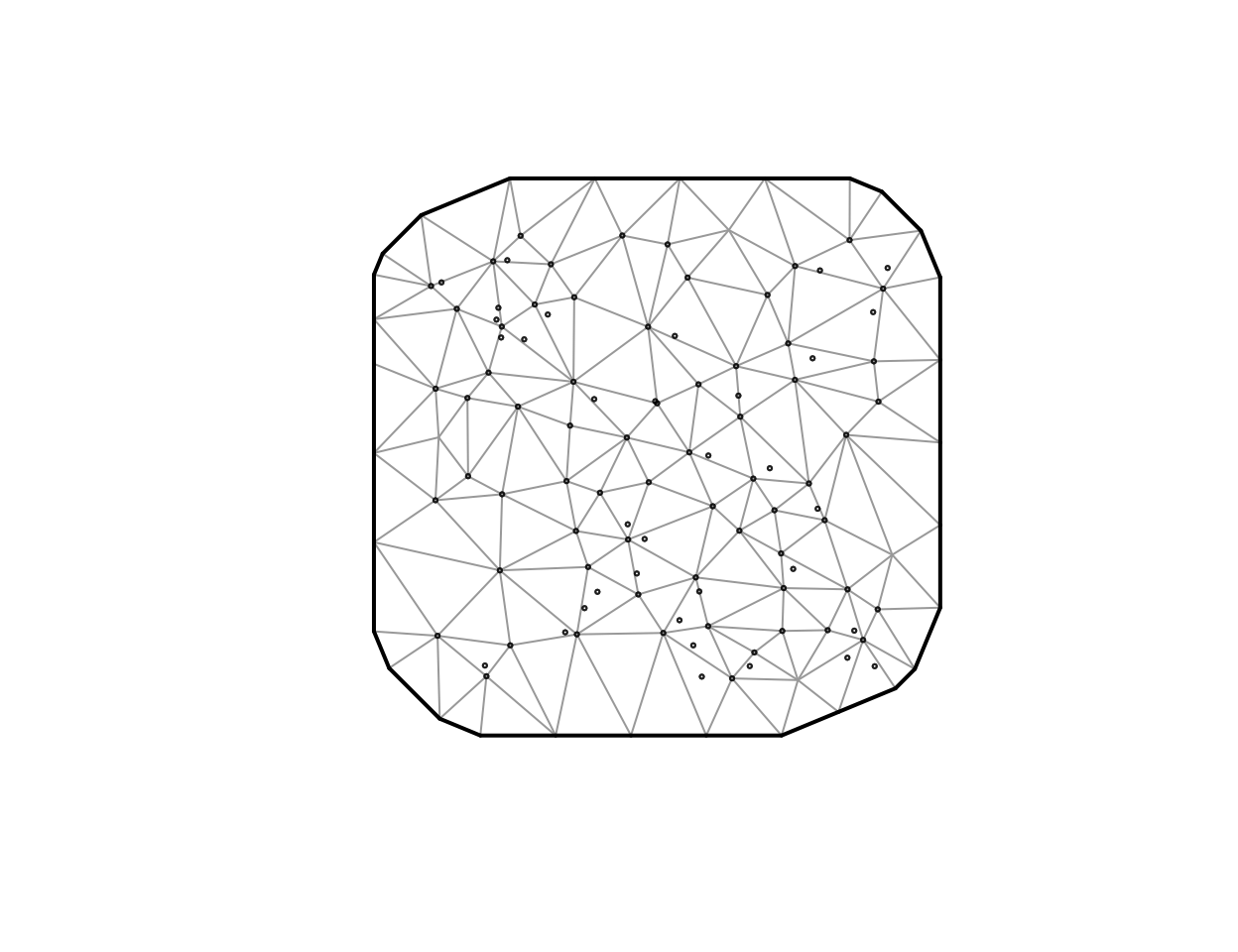

Triangulated mesh of many small triangles covering a scatter of site locations, with a coarser buffer of triangles around the edge.

SPDE mesh triangulating the simulated sites: edges show the triangulation, vertices carry the spatial field. Axes are in the site coordinate units.

Inspect the mesh before fitting. It should cover every sampling location without a fringe of extremely narrow triangles. A mesh that is too coarse can erase short-range structure; a needlessly fine mesh adds latent variables and can make optimization slower.

The projection matrix must follow the rows used by the model. The long data already have that order. If your data start wide, make an equivalent row-major coordinate frame before calling make_mesh():

trait_cols <- c("trait_1", "trait_2", "trait_3")
mesh_data <- spatial_wide[
  rep(seq_len(nrow(spatial_wide)), each = length(trait_cols)),
  c("lon", "lat"),
  drop = FALSE
]
mesh <- make_mesh(mesh_data, c("lon", "lat"), cutoff = 0.07)

This explicit alignment protects against the most consequential mesh failure: a projection matrix whose rows no longer correspond to the fitted response cells.

Fit the same model in long and wide form

For trait $t$ at site $i$ , the worked model is $y_{it} = \alpha_t + u_t(s_i) + \varepsilon_{it}$ . The fields $u_t$ are independent across traits. Their shared mesh geometry is represented by

$Q(\kappa) = \kappa^4 M_0 + 2\kappa^2 M_1 + M_2,$

where the mesh supplies $M_0$ , $M_1$ , and $M_2$ . The parameter $\kappa$ controls the practical range; trait-specific scale parameters control how strongly each field varies.

fit_long <- gllvmTMB(
  value ~ 0 + trait + spatial_indep(0 + trait | site),
  data = spatial_long,
  trait = "trait",
  unit = "site",
  mesh = mesh,
  silent = TRUE
)

Some readers store one response column per trait. The compact traits() formula uses spatial_indep(1 | site); the formula expander creates the same trait-specific intercept and spatial-field design as the long call.

spatial_wide <- reshape(
  spatial_long[c("site", "lon", "lat", "trait", "value")],
  idvar = c("site", "lon", "lat"),
  timevar = "trait",
  direction = "wide"
)
names(spatial_wide) <- sub("value.", "", names(spatial_wide), fixed = TRUE)
row.names(spatial_wide) <- NULL

fit_wide <- gllvmTMB(
  traits(trait_1, trait_2, trait_3) ~
    1 + spatial_indep(1 | site),
  data = spatial_wide,
  unit = "site",
  mesh = mesh,
  silent = TRUE
)

c(
  long_convergence = fit_long$opt$convergence,
  wide_convergence = fit_wide$opt$convergence,
  long_logLik = unname(logLik(fit_long)),
  wide_logLik = unname(logLik(fit_wide))
)
#> long_convergence wide_convergence      long_logLik      wide_logLik 
#>           0.0000           0.0000        -431.4045        -431.4045

The two calls are alternative data interfaces, not different statistical models. Use long data when trait labels are already rows; use traits() when the responses are columns.

Interpret the practical range

The current spatial engine assumes isotropy: dependence changes with distance but not direction. plot_anisotropy() therefore displays a circle and reports the fitted practical range; it does not estimate directional anisotropy.

data.frame(
  true_range = spatial_sim$truth$spatial_range,
  fitted_range = sqrt(8) / as.numeric(fit_long$report$kappa[1]),
  assumption = "isotropic (H = I)"
)
#>   true_range fitted_range        assumption
#> 1        0.3    0.2216269 isotropic (H = I)

invisible(plot_anisotropy(fit_long))

The fitted value is one point estimate from one simulated dataset. Agreement with the generating value is a teaching check, not evidence of unbiased range estimation or calibrated uncertainty across designs.

Absolute spatial field scale is also not validated. Treat fitted tau, field SD, and projected marginal SD as exploratory model-based point estimates; do not present them as recovered absolute scale or calibrated uncertainty. Those estimands require a separate fixed-range and estimated-range recovery study.

Run the ordinary fit diagnostics before interpreting spatial parameters — look for the same optimizer_convergence / pd_hessian pair used throughout this series:

health <- check_gllvmTMB(fit_long)
health[health$component %in% c("optimizer_convergence", "pd_hessian"),
       c("component", "status")]
#>               component status
#> 1 optimizer_convergence   PASS
#> 4            pd_hessian   PASS

Choose the spatial covariance mode

The current spatial modes use the same mesh and SPDE geometry. They differ in the trait covariance allowed for the spatial field.

Keyword	Spatial covariance question
`spatial_indep(..., common = TRUE)`	Should all traits have one common spatial-field variance, with no cross-trait spatial covariance?
`spatial_indep()`	Should traits have separate spatial-field variances but zero cross-trait spatial covariance?
`spatial_latent(..., d = K)`	Can $K$ shared spatial axes describe cross-trait spatial covariance?
`spatial_dep()`	Should the model estimate a full cross-trait spatial covariance?

spatial_scalar() is retained as soft-deprecated compatibility syntax for the first row. Use spatial_indep(..., common = TRUE) in new code.

Start with the simplest mode that answers the biological question. Do not add spatial_indep() to spatial_latent() or spatial_dep() in the same formula; those combinations duplicate spatial variance and fail explicitly.

Fit the reduced-rank and full-covariance alternatives by changing only the spatial term:

fit_latent <- gllvmTMB(
  value ~ 0 + trait +
    spatial_latent(0 + trait | site, d = 2, unique = TRUE),
  data = spatial_long,
  trait = "trait",
  unit = "site",
  mesh = mesh,
  silent = TRUE
)

fit_dep <- gllvmTMB(
  value ~ 0 + trait + spatial_dep(0 + trait | site),
  data = spatial_long,
  trait = "trait",
  unit = "site",
  mesh = mesh,
  silent = TRUE
)

The matching wide-data formulas are unevaluated structural translations. They reuse the stacked mesh-coordinate construction shown above, but this article does not demonstrate long/wide fit parity for either correlated alternative:

fit_latent_wide <- gllvmTMB(
  traits(trait_1, trait_2, trait_3) ~
    1 + spatial_latent(1 | site, d = 2, unique = TRUE),
  data = spatial_wide,
  unit = "site",
  mesh = mesh,
  silent = TRUE
)

fit_dep_wide <- gllvmTMB(
  traits(trait_1, trait_2, trait_3) ~ 1 + spatial_dep(1 | site),
  data = spatial_wide,
  unit = "site",
  mesh = mesh,
  silent = TRUE
)

mode	log_likelihood	AIC
indep	-431.4	878.8
latent (d = 2, unique = TRUE)	-426.5	878.9
dep	-426.5	874.9

Here d = 2 requests two shared spatial axes, while unique = TRUE retains a trait-specific spatial diagonal, so $\Sigma_{\mathrm{spatial}} = \Lambda_{\mathrm{spatial}} \Lambda_{\mathrm{spatial}}^\top + \Psi_{\mathrm{spatial}}$ . As with every loading matrix in this package, the rotation and sign of $\Lambda_{\mathrm{spatial}}$ are arbitrary. In this three-trait rank-two example, however, the split between $\Lambda\Lambda^\top$ and $\Psi_{\mathrm{spatial}}$ is also not unique beyond those rotations: different shared diagonals and positive diagonal $\Psi_{\mathrm{spatial}}$ values can give the same total spatial covariance. For example, the loading rows $(1,0),\ (1/2,1),\ (1/2,1/2)$ and $(\sqrt{2},0),\ (1/(2\sqrt{2}),1),\ (1/(2\sqrt{2}),5/8)$ both give off-diagonals $(1/2,1/2,3/4)$ , but their shared diagonals are $(1,5/4,1/2)$ and $(2,9/8,33/64)$ . Different positive diagonal Psi companions can bring the total diagonal to $(3,3,3)$ in each decomposition. This is a structural decomposition ambiguity, not a failed fit. Interpret shared axes and communality as decomposition-sensitive; the total spatial covariance is the intended covariance target. spatial_dep() estimates the full cross-trait spatial covariance. The data were generated with independent trait fields, so this table demonstrates runnable syntax and relative fit on one dataset; it is not a recovery or model-selection study. These broader models remain only partially validated — both the wider spatial-keyword family and this paired latent/unique total-covariance route lack full recovery evidence — so treat current estimates as model-based point estimates rather than calibrated spatial-correlation inference.

Provenance, acknowledgement, and licensing

gllvmTMB does not import, link to, or include sdmTMB; sdmTMB is not a runtime or build dependency. The original gllvmTMB spatial interface and helper layer were derived from sdmTMB’s GPL-3 implementation. Repository history and inst/COPYRIGHTS retain that attribution.

The current helpers in R/mesh.R, R/crs.R, and R/plot.R were substantially rewritten for gllvmTMB from the published SPDE/GMRF construction and the public fmesher API. They remain distributed under GPL-3, which is compatible with their sdmTMB source lineage. The repository records the detailed code-provenance boundary in inst/COPYRIGHTS.

Users should cite gllvmTMB and TMB through citation("gllvmTMB"). The sdmTMB acknowledgement does not create a separate required citation for using these substantially rewritten helpers.

What to do next

If your question is…	Continue with…
Which spatial covariance mode matches my estimand?	Formula keyword grid
Do species still co-occur after environmental predictors?	Joint species distribution models
Can I trust this fitted object numerically?	Fit diagnostics
How does the SPDE keyword map to the engine?	`spatial_indep()` reference

Single-response spatial models belong in sdmTMB. Directional anisotropy, barrier meshes, and spatiotemporal fields are not implemented in the current gllvmTMB spatial helper contract.

References

Lindgren F, Rue H, Lindström J (2011). An explicit link between Gaussian fields and Gaussian Markov random fields: the stochastic partial differential equation approach. Journal of the Royal Statistical Society: Series B, 73, 423–498. https://doi.org/10.1111/j.1467-9868.2011.00777.x.