Start here: which species distribution model do your data allow?

You have some species records and a question about where things live. The species distribution literature will offer you a dozen model names, and it is not obvious which of them your data entitle you to. This page is the shortest route from what is in your spreadsheet to which article to open.

It is a hallway, not a room. Nothing is fitted here. Everything below runs on base R alone, in a couple of seconds, so you can paste it into a console and see the pictures for yourself. When an article does ask you to fit something, the package installs straight from GitHub:

# install.packages("remotes")
remotes::install_github("itchyshin/gllvmTMB")

The routes on this site do not all estimate one ecological quantity. Keep three targets separate before choosing a model:

Abundance or intensity describes how many individuals, records, or events are expected per unit of effort or sampled support. The count and integrated routes here estimate relative ecological intensity: where it is higher or lower, not absolute abundance.
Occurrence or observation probability is a probability between zero and one. The ordinary binary JSDM models $P(Y=1)$ for a species-site cell. That can be called occurrence probability only when the survey design makes a 1 a record of occurrence and assumes no separate imperfect-detection process; otherwise it is the probability of an observed 1 under that protocol.
A detection process asks for the chance of observing a species given that it is present. Separating that chance from occurrence requires repeat visits and an occupancy model with a detection submodel. Neither the single-visit binary JSDM nor the integrated route on this site estimates detectability.

The illustration below uses one shared-intensity scenario so the four data windows can be compared on common ground. This is the specific construction used by the package’s integrated Poisson and complementary-log-log routes, not a claim that every SDM targets intensity. What you observe is decided by how the data were collected:

Counts with effort — a checklist, a trap-night, a timed transect — are random counts whose expected value scales with intensity and how hard you looked. Doubling known effort doubles the expected count, not every realized count.
Detection / non-detection is a random 0/1 outcome. In the integrated shared-intensity route, a visit with support $a$ and intensity $\lambda$ has $P(Y=1)=1-\exp(-a\lambda)$ : a low-intensity site can still produce a 1 and a high-intensity site can still produce a 0. The binary result does not report how many individuals or records were available.
Presence-only records — one photo, one point, uploaded by a stranger — see the surface through a second filter: where people go. A road, a car park, and a popular reserve all look like good habitat.
Grid cells see the surface averaged over squares. Averaging flattens peaks; a hotspot smaller than a cell stops existing.

A five-panel figure. The large central panel is a smooth relative-intensity surface on a viridis scale with white contour lines, showing a large bright peak in the upper left and a smaller peak in the lower right against a dark background. Four smaller white panels flank it. Panel a shows random counts as printed numbers, with larger counts more common in the upper-left region and text size showing effort. Panel b shows one random binary draw per site as circles, mostly filled in the upper left but with both outcomes possible across the surface. Panel c shows presence-only records as plus signs forming two clumps, one on the upper-left ecological peak and a denser one in the accessible lower-right corner. Panel d shows a five-by-five grid of coloured squares on the same scale as the central panel, with the peak reduced to a single mid-bright square.

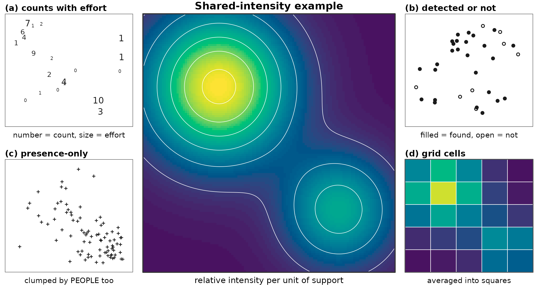
One simulated shared-intensity landscape, seen four ways. The centre panel is relative intensity per unit of support, which no data type observes directly; the flanking panels show one random realization from each observation window. (a) counts at twenty places, printed as numbers, with text size marking how much effort each place received. (b) one Bernoulli detection/non-detection draw at each of thirty-four places: filled circles are 1 and open circles are 0, with probability 1 - exp(-intensity) rather than a deterministic intensity threshold. (c) eighty-five presence-only records, proposed where people are and then thinned by intensity, so they pile up both on the ecological hotspot and in the accessible bottom-right corner. (d) the same intensity averaged into twenty-five coarse cells on the same colour scale, which visibly drains the bright peak. This is a drawn illustration on simulated data, not a fitted model and not a claim that every route estimates intensity.

The consequence is the single most useful idea on this site: the model you need is not chosen by your species or your region — it is chosen by your window. Two people studying the same warbler in the same valley need different models if one of them has checklists and the other has photographs.

Combining sources can be worth the trouble, but it is not automatically more informative. It can improve identification or precision when the sources can validly share an ecological state, their effort and observation biases are represented, and their spatial support is compatible. It can instead add bias or conflict when those assumptions fail. The integrated route on this site therefore admits a narrow pairing: Poisson counts and Bernoulli-cloglog 0/1 observations that can both be written as thinnings of one shared relative intensity, with each source retaining its own observation law. It does not turn that shared intensity into absolute abundance, occupancy, or detectability.

Two questions decide your route

What do you have? (the window) and what do you want to know? (the question). The tree answers the first; the table underneath adds the second.

A flow chart reading top to bottom. A grey box at the top reads: what do your data look like? Four arrows lead to four boxes: presence-only records; counts with effort; detection or non-detection with one visit per place; and repeat-visit histories. The presence-only box leads to a diamond asking whether the question is a trend over years, whose yes branch reaches a dashed box reading grid cells plus list-based occupancy models, and whose no branch reaches a solid box reading joint intensity from records, counted per grid cell. Counts with effort leads straight to a solid box reading joint intensity from records, count arm, no recording-bias term. Detection or non-detection leads straight to a solid box reading binary joint SDM, with one observed-1 probability and no occurrence/detection split. Repeat-visit histories leads to a diamond asking whether occurrence must be split from detection, whose yes branch reaches a dashed box reading spOccupancy carries the detection submodel, and whose no branch reaches a solid box reading what repeat visits add to one shared intensity. Dotted lines gather the compatible source boxes into a wide band at the foot reading: have two or more compatible sources at once? That is the integrated model, one shared relative intensity with each source keeping its own observation law.

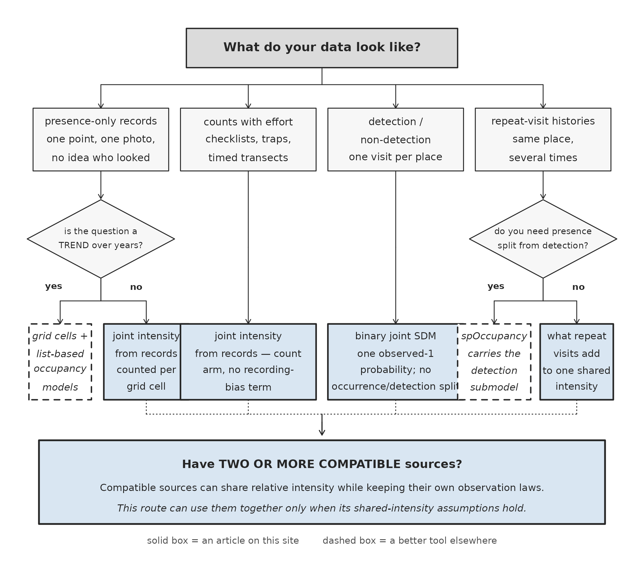
Routing by data type. Read downwards: the top row is what your data look like, the diamonds are the two follow-up questions where the answer sends you off this site, and the bottom row is a destination. Solid boxes are articles here; dashed boxes are honest exits to a better tool elsewhere, distinguished by border style rather than by colour so the distinction survives greyscale printing. The band along the foot applies when two or more sources satisfy the shared-intensity assumptions described in the text.

The tree routes on data alone. Your question splits the destinations further:

you have ↓ / you want →	a map, or a habitat response	community structure — which species covary	“was it really there?” — detection separated
counts with effort checklists, traps, transects	joint intensity from records, count arm (an arm = one data source in a joint fit) · add space	the same fit — all species respond to a few shared, unmeasured gradients	not from counts alone; you need repeat visits
detection / non-detection one visit per place	binary joint SDM · or its survey arm	binary joint SDM · if a species is too rare	not possible from one visit — the occupancy model collapses into this one
detection histories repeat visits	what repeat visits add — but read the exit first	possible, same fit	spOccupancy territory — see the honest exits
presence-only one photo, one point	joint intensity from records — records counted per grid cell. For the point-process treatment (each record a location, with background points) see the recipe in the Warbler article	the same fit	the occupancy-trend tradition — see the honest exits
mixed sources eBird plus your own survey	the integrated model, end to end · start smaller · go wider	yes, and it is the same fit	only as far as the survey arm’s visits allow

Two honesty notes about that table. There is no article here devoted to counts from a single designed survey; the machinery for it lives inside the presence-only article, because a designed count uses the same Poisson likelihood with the recording-bias term switched off. Those count and integrated routes return relative intensity, not absolute abundance, occupancy probability, or detectability. The ordinary binary JSDM instead models $P(Y=1)$ with a binomial link. With one visit and no detection submodel, that fitted probability cannot be decomposed into occurrence and detection. The individual articles state the interpretation boundary for each route.

The honest exits

Some questions are better answered elsewhere. Saying so is part of the routing.

One species, not many. Everything on this site is built for many species at once — that is the whole point of the shared surfaces and the latent gradients. If you have a single species, you are paying for machinery you do not need. Use sdmTMB, which fits single-response spatial and spatiotemporal models with the same underlying technology (TMB with SPDE meshes), is on CRAN, and — unlike this package today — gives you uncertainty on its predictions. It is also the package this one’s mesh and coordinate helpers descend from: make_mesh() and add_utm_columns() will look familiar because they are, by lineage (see inst/COPYRIGHTS). The dividing line is simple: one response, use sdmTMB; several responses sharing structure, come back here.

Integrated models in the INLA tradition. The integration on this site is one way of doing it. PointedSDMs and intSDM build integrated species distribution models on INLA/inlabru instead, and are the better starting point if your lab already works that way or you want a single-species integrated fit.

Occupancy models. These separate two probabilities: occurrence and a detection submodel, the chance of observing the species given that it is present. Repeat visits supply the within-site detection history needed to estimate that split. If you have repeat visits and your question genuinely needs “was it there” separated from “did we find it” — absolute occupancy, or a long-term trend from opportunistic data — use spOccupancy, which is built for exactly that. With a single visit, occurrence and detection are not separately identified. The binary JSDM here fits the resulting observed-1 probability as one quantity; it does not estimate an occupancy/detection decomposition.

Trends from one-photo records, the way insect recording schemes work. The established route is grid cells plus occupancy modelling of list-based visits — using the other species recorded on the same list to reconstruct the visit and detection structure a raw photo stream lacks (van Strien, van Swaay and Termaat 2013, Opportunistic citizen science data of animal species produce reliable estimates of distribution trends if analysed with occupancy models). Not this package. This package’s presence-only route is aimed at habitat responses and intensity maps, not at trends.

Uncertainty on a map. The prediction maps produced here currently carry no intervals of any kind — predict() refuses se.fit with new data rather than returning a number that ignores the dominant source of error. If your thesis figure needs a confidence interval on every pixel, that is a real limit of this package today, and you should know it before you build a chapter on it. The Canada Warbler article states the point in full, and Current limitations keeps the running list.

Where to start reading

A short path, in order.

What is a site? The unit of analysis — before anything else. It settles the data-shape decisions that every route below inherits, and it will probably talk you out of gridding your data.
Your cell of the table above. One article. Fit the toy example in it before you touch your own data.
The two warning articles, before real data. When one data source knows where it is and the other does not is about location precision, which decides whether combining sources helps or hurts. And the “Before you use this on real data” section of the Canada Warbler article is the checklist of things that go wrong first.

If a word on any of those pages is unfamiliar, the plain-English vocabulary page defines the package’s terms in one line each. If you are sizing a survey rather than analysing one, How much survey do you need? is the page for that.

The integrated route on this site is experimental: the interface is settled enough to use and the estimates are illustrated on known-truth simulations, but confidence intervals for it are not certified. Each article says where its own evidence stops.

How the figures were drawn

Both figures use only base R and take about a second. Nothing in them is fitted; they draw one shared-intensity observation scenario and the resulting reader routes.

set.seed(7)

## One smooth surface: relative intensity per unit of support on a unit square.
## Nothing here is a fit -- this is one shared-intensity scenario, not a claim
## that all species-distribution models target the same quantity.
lambda <- function(x, y) {
  6.0 * exp(-((x - 0.30)^2 + (y - 0.72)^2) / 0.075) +
  3.2 * exp(-((x - 0.78)^2 + (y - 0.24)^2) / 0.045) + 0.35
}
gx <- seq(0, 1, length.out = 120); gy <- gx
Z  <- outer(gx, gy, lambda)

pal  <- hcl.colors(64, "Viridis")       # monotone luminance: survives greyscale
brks <- seq(0, max(Z) * 1.001, length.out = 65)
ins  <- function(n) 0.08 + 0.84 * runif(n)   # keep marks off the panel border

## (a) counts with effort: where you looked, and how hard.
n_a <- 20; ax <- ins(n_a); ay <- ins(n_a)
eff <- sample(c(0.4, 1, 2), n_a, replace = TRUE)
cnt <- rpois(n_a, lambda(ax, ay) * eff)

## (b) detection / non-detection at one visit per place.
n_b <- 34; bx <- ins(n_b); by <- ins(n_b)
det <- rbinom(n_b, 1, 1 - exp(-lambda(bx, by)))

## (c) presence-only: proposed where PEOPLE go, then thinned by the surface.
n_c  <- 85
cand <- cbind(ins(4000), ins(4000))
wt   <- exp(-sqrt((cand[, 1] - 0.94)^2 + (cand[, 2] - 0.06)^2) / 0.26) *
        lambda(cand[, 1], cand[, 2])
kp   <- sample(nrow(cand), n_c, prob = wt)
cx   <- cand[kp, 1]; cy <- cand[kp, 2]

## (d) the same surface averaged over 5 x 5 coarse cells.
K <- 5; ex <- seq(0, 1, length.out = K + 1)
Zc <- outer(seq_len(K), seq_len(K), Vectorize(function(i, j)
  mean(Z[gx >= ex[i] & gx < ex[i + 1], gy >= ex[j] & gy < ex[j + 1]])))

blank <- function() {
  plot.new(); plot.window(c(0, 1), c(0, 1), xaxs = "i", yaxs = "i")
  rect(0, 0, 1, 1, col = "white", border = "grey30")
}
tag <- function(lab, sub) {
  mtext(lab, side = 3, line = 0.10, adj = 0, cex = 0.68, font = 2)
  mtext(sub, side = 1, line = 0.30, cex = 0.60)
}

op <- par(no.readonly = TRUE)
layout(matrix(c(2, 1, 1, 3,
                4, 1, 1, 5), nrow = 2, byrow = TRUE),
       widths = c(1, 0.95, 0.95, 1))
par(mar = c(1.9, 0.5, 1.4, 0.5))

## The centre: the surface itself.
image(gx, gy, Z, col = pal, breaks = brks, axes = FALSE, xlab = "", ylab = "",
      xaxs = "i", yaxs = "i")
contour(gx, gy, Z, add = TRUE, drawlabels = FALSE, col = "white", lwd = 0.6,
        levels = pretty(range(Z), 6))
box(col = "grey20", lwd = 1.4)
mtext("Shared-intensity example", side = 3, line = 0.25, cex = 0.82, font = 2)
mtext("relative intensity per unit of support", side = 1,
      line = 0.30, cex = 0.66)

blank(); text(ax, ay, cnt, cex = 0.60 + 0.20 * log2(eff * 2.5), col = "grey10")
tag("(a) counts with effort", "number = count, size = effort")

blank(); points(bx, by, pch = ifelse(det == 1, 19, 1), cex = 0.82,
                col = "grey10", lwd = 1.1)
tag("(b) detected or not", "filled = found, open = not")

blank(); points(cx, cy, pch = 3, cex = 0.52, col = "grey10", lwd = 0.9)
tag("(c) presence-only", "clumped by PEOPLE too")

image(ex, ex, Zc, col = pal, breaks = brks, axes = FALSE, xlab = "", ylab = "",
      xaxs = "i", yaxs = "i")
abline(v = ex, h = ex, col = "white", lwd = 0.7); box(col = "grey30")
tag("(d) grid cells", "averaged into squares")
par(op)

op <- par(no.readonly = TRUE)
par(mar = c(0.2, 0.2, 0.2, 0.2))
plot.new(); plot.window(xlim = c(0, 100), ylim = c(0, 100))

INK <- "grey15"

## A box. `kind` sets the border STYLE as well as the fill, so the distinction
## between "an article on this site" and "a better tool elsewhere" survives
## printing in greyscale: destinations are solid, honest exits are dashed.
bx <- function(x, y, w, h, txt, kind = "branch", gap = 3.4) {
  sty <- switch(kind,
    start  = list(fill = "grey86", lty = 1, lwd = 1.4, font = 2, cex = 0.82),
    branch = list(fill = "grey97", lty = 1, lwd = 1.0, font = 1, cex = 0.68),
    leaf   = list(fill = "#D9E6F2", lty = 1, lwd = 1.7, font = 1, cex = 0.66),
    exit   = list(fill = "white",   lty = 2, lwd = 1.5, font = 3, cex = 0.66))
  rect(x - w/2, y - h/2, x + w/2, y + h/2, col = sty$fill,
       border = INK, lty = sty$lty, lwd = sty$lwd)
  n <- length(txt)
  text(x, y + (n - 1)/2 * gap - (seq_len(n) - 1) * gap,
       txt, cex = sty$cex, font = sty$font, col = INK)
}

dia <- function(x, y, w, h, txt) {
  polygon(c(x - w/2, x, x + w/2, x), c(y, y + h/2, y, y - h/2),
          col = "grey97", border = INK, lwd = 1.0)
  n <- length(txt)
  text(x, y + (n - 1)/2 * 2.7 - (seq_len(n) - 1) * 2.7,
       txt, cex = 0.59, col = INK)
}

## Elbow connector: down out of the parent, across, then down into the child.
elb <- function(x0, y0, x1, y1, lab = NULL, lx = 0) {
  ym <- (y0 + y1) / 2
  segments(x0, y0, x0, ym, col = INK, lwd = 0.9)
  segments(x0, ym, x1, ym, col = INK, lwd = 0.9)
  arrows(x1, ym, x1, y1, length = 0.055, col = INK, lwd = 0.9)
  if (!is.null(lab)) text(x0 + lx, (y0 + ym)/2 + 0.4, lab,
                          cex = 0.60, font = 2, col = INK)
}

## ---- the tree, read downwards ---------------------------------------------
bx(50, 95.5, 46, 7.5, "What do your data look like?", "start")

cxs <- c(12.5, 37.5, 62.5, 87.5)
bx(cxs[1], 78, 23, 12, c("presence-only records", "one point, one photo,", "no idea who looked"), "branch")
bx(cxs[2], 78, 23, 12, c("counts with effort", "checklists, traps,", "timed transects"), "branch")
bx(cxs[3], 78, 23, 12, c("detection /", "non-detection", "one visit per place"), "branch")
bx(cxs[4], 78, 23, 12, c("repeat-visit histories", "same place,", "several times"), "branch")

segments(50, 91.75, 50, 88.5, col = INK, lwd = 0.9)
segments(cxs[1], 88.5, cxs[4], 88.5, col = INK, lwd = 0.9)
for (x in cxs) arrows(x, 88.5, x, 84.0, length = 0.055, col = INK, lwd = 0.9)

## A follow-up question only where an honest exit lives.
dia(cxs[1], 59, 25, 15, c("is the question a", "TREND over years?"))
dia(cxs[4], 59, 25, 15, c("do you need presence", "split from detection?"))
for (x in c(cxs[1], cxs[4])) arrows(x, 72, x, 66.7, length = 0.055, col = INK, lwd = 0.9)

## Leaves. Solid = an article here; dashed = somebody else's tool.
bx( 5.6, 35.5, 10.6, 14.5, c("grid cells +", "list-based", "occupancy", "models"), "exit", 3.2)
bx(20.2, 35.5, 14.4, 14.5, c("joint intensity", "from records", "counted per", "grid cell"), "leaf", 3.2)
bx(cxs[2], 35.5, 23, 14.5, c("joint intensity", "from records — count", "arm, no recording-", "bias term"), "leaf", 3.2)
bx(cxs[3], 35.5, 23, 14.5, c("binary joint SDM", "one observed-1", "probability; no", "occurrence/detection split"), "leaf", 3.2)
bx(79.2, 35.5, 12.4, 14.5, c("spOccupancy", "carries the", "detection", "submodel"), "exit", 3.2)
bx(93.2, 35.5, 12.4, 14.5, c("what repeat", "visits add", "to one shared", "intensity"), "leaf", 3.2)

elb(cxs[1], 51.5,  5.6, 42.8, "yes", -8.0)
elb(cxs[1], 51.5, 20.2, 42.8, "no",   6.0)
elb(cxs[4], 51.5, 79.2, 42.8, "yes", -8.0)
elb(cxs[4], 51.5, 93.2, 42.8, "no",   6.0)
elb(cxs[2], 72.0, cxs[2], 42.8)
elb(cxs[3], 72.0, cxs[3], 42.8)

## The band. Only the SOLID leaves feed it; the exits deliberately do not.
for (x in c(20.2, cxs[2], cxs[3], 93.2))
  segments(x, 28.25, x, 25.5, col = INK, lwd = 0.9, lty = 3)
segments(20.2, 25.5, 93.2, 25.5, col = INK, lwd = 0.9, lty = 3)
segments(50, 25.5, 50, 22.5, col = INK, lwd = 1.1)
arrows(50, 24, 50, 21.5, length = 0.06, col = INK, lwd = 1.1)

rect(2, 4.5, 98, 20.5, col = "#D9E6F2", border = INK, lwd = 1.9)
text(50, 16.0, "Have TWO OR MORE COMPATIBLE sources?", cex = 0.78, font = 2, col = INK)
text(50, 11.3, "Compatible sources can share relative intensity while keeping their own observation laws.",
     cex = 0.66, col = INK)
text(50,  7.4, "This route can use them together only when its shared-intensity assumptions hold.",
     cex = 0.66, font = 3, col = INK)

## Legend, parked below everything so it can collide with nothing.
text(50, 1.4, "solid box = an article on this site        dashed box = a better tool elsewhere",
     cex = 0.62, col = "grey30")
par(op)

What this is built on

None of this is new from nothing. The pieces this package stands on, and what each of them gave it:

TMB (Kristensen et al. 2016) — automatic differentiation and the Laplace approximation. Every fit on this site is a TMB fit; without it none of these models would be practical in R.
glmmTMB (Brooks et al.
1. — the mixed-model formula grammar and family machinery that this package’s interface follows, so that a user who knows glmmTMB already knows most of this.
sdmTMB (Anderson et al. 2025) — the SPDE and mesh layer. make_mesh(), add_utm_columns() and the spatial interface here descend directly from sdmTMB’s GPL-3 implementation, with the provenance recorded in inst/COPYRIGHTS. It remains the right package for single-species spatial models, and it does things this one does not — prediction uncertainty and spatiotemporal fields among them.
gllvm (Niku et al. 2019) — the generalised linear latent variable model for community ecology, the statistical idea this package extends rather than invents.
fmesher and the INLA/SPDE literature (Lindgren, Rue and Lindström 2011) — the representation of a continuous spatial field on a triangulated mesh.
The point-process tradition in ecology — Warton and Shepherd (2010) and Renner et al. (2015), who established that presence-only data are point patterns and that fitting them as a weighted Poisson regression is both principled and practical.

Where this package differs from its predecessors, it says so; where it borrows, it says that too. Building on other people’s work is how the field moves, and the borrowing is worth naming rather than hiding.

References