
How many latent dimensions should I fit?
Source:vignettes/articles/model-selection-latent-rank.Rmd
model-selection-latent-rank.RmdBefore interpreting a latent variable (LV), choose the rank you are willing to defend. This article asks a practical question: when the same multi-trait data can be fitted with one, two, or more latent variables (LVs), how do AIC, BIC, fit health, and biological interpretability help decide which model to report?
This is model-based rank selection — comparing penalised marginal likelihoods of fitted GLLVMs — not a PCA or NMDS scree rule that picks dimensions by variance explained. The LVs here are random effects of a fitted covariance model (below), not an eigen-decomposition of the raw data, so “how many LVs?” is answered by penalised likelihood and fit health rather than a scree plot or a variance-explained cutoff.
The criteria and recovery numbers below orient a workflow on one simulated fixture; they are not backed by a repeated-sampling coverage study for this target.
The example simulates five continuous traits with two planted latent
variables. We fit candidate ranks with gllvmTMB(), compare
their information criteria, check numerical health, and interpret the
chosen model as a rank-conditional summary rather than proof that nature
has exactly two hidden LVs.
A safe reporting order is: first check numerical and response diagnostics; next compare one ML candidate set with AIC/BIC; then interpret rotation-invariant summaries for the chosen rank; finally, for Gaussian fits only, refit that chosen model with REML for covariance summaries. The REML log-likelihood is not part of the ML AIC/BIC table.
Start With One Data Problem
The fixture has one row per (individual, trait)
observation. The traits are continuous measurements with a planted
size axis and a planted shape axis. The true
between-individual covariance is
where Lambda contains the shared latent loadings and
Psi is the trait-specific diagonal carried by ordinary
latent().
rank_ex <- readRDS(system.file(
  "extdata", "examples", "model-selection-rank-example.rds",
  package = "gllvmTMB"
))
df <- rank_ex$data_long
df_wide <- rank_ex$data_wide
truth <- rank_ex$truth
rank_ex$story$question
#> [1] "Do five continuous traits need one latent axis, two axes, or a richer rank before the covariance summary is interpretable?"
head(df, 8)
#>   individual  trait      value
#> 1          1 length -0.7366122
#> 2          1   mass -0.1850625
#> 3          1   wing -0.1015537
#> 4          1 tarsus -0.7591717
#> 5          1   bill -0.4639405
#> 6          2 length  0.5835341
#> 7          2   mass  1.4148848
#> 8          2   wing  0.8739607
round(truth$Lambda, 2)
#>        size shape
#> length  0.9   0.1
#> mass    1.0   0.2
#> wing    0.8  -0.4
#> tarsus  0.7  -0.5
#> bill    0.6   0.6
The planted d = 2 truth is only a teaching fixture. In
real data, the rank is unknown; the candidate set is a set of defensible
summaries, not a direct view into biological machinery.
The long and wide versions of the selected-rank formula are:
rank_ex$formula_long
#> value ~ 0 + trait + latent(0 + trait | individual, d = 2)
rank_ex$formula_wide
#> traits(length, mass, wing, tarsus, bill) ~ 1 + latent(1 | individual,
#>     d = 2)
Fit Candidate Ranks
The diagonal baseline has no shared latent variable, so it uses
indep(). The d >= 1 candidates use the same
fixed effects and ordinary latent() decomposition, changing
only the rank of the shared Lambda Lambda^T term.
candidate_formula <- function(d) {
  if (identical(d, 0L)) {
    return(value ~ 0 + trait + indep(0 + trait | individual))
  }

  stats::as.formula(paste0(
    "value ~ 0 + trait + ",
    "latent(0 + trait | individual, d = ", d, ")"
  ))
}

fit_candidate <- function(d, data, control) {
  suppressMessages(suppressWarnings(gllvmTMB(
    candidate_formula(d),
    data = data,
    trait = "trait",
    unit = "individual",
    family = gaussian(),
    control = control
  )))
}

summarise_candidate <- function(fit, d) {
  ll <- logLik(fit)
  health <- check_gllvmTMB(fit)
  weak_axis <- health[health$component == "weak_axis_unit", , drop = FALSE]
  health_status <- if (any(health$status == "FAIL")) {
    "FAIL"
  } else if (any(health$status == "WARN")) {
    "WARN"
  } else {
    "PASS"
  }

  data.frame(
    d = d,
    model = if (d == 0L) "indep only" else paste0("latent d = ", d),
    logLik = as.numeric(ll),
    df = attr(ll, "df"),
    nobs = attr(ll, "nobs"),
    AIC = AIC(fit),
    BIC = BIC(fit),
    convergence = fit$opt$convergence,
    pd_hessian = isTRUE(fit$fit_health$pd_hessian),
    max_gradient = fit$fit_health$max_gradient,
    weak_axis = if (nrow(weak_axis)) weak_axis$status[1] else "not fitted",
    health = health_status,
    stringsAsFactors = FALSE
  )
}
candidate_d <- 0:3
rank_control <- gllvmTMBcontrol(n_init = 2, init_jitter = 0.02)

fits <- setNames(
  lapply(candidate_d, fit_candidate, data = df, control = rank_control),
  paste0("d", candidate_d)
)

rank_table <- do.call(
  rbind,
  lapply(candidate_d, function(d) summarise_candidate(fits[[paste0("d", d)]], d))
)
rank_table$delta_AIC <- rank_table$AIC - min(rank_table$AIC)
rank_table$delta_BIC <- rank_table$BIC - min(rank_table$BIC)

rank_table_display <- rank_table[
  , c(
    "model", "logLik", "df", "nobs", "AIC", "BIC",
    "delta_AIC", "delta_BIC", "pd_hessian", "weak_axis", "health"
  )
]
rank_table_display[, c("logLik", "AIC", "BIC", "delta_AIC", "delta_BIC")] <-
  round(rank_table_display[, c("logLik", "AIC", "BIC", "delta_AIC", "delta_BIC")], 1)
rank_table_display
#>          model logLik df nobs    AIC    BIC delta_AIC delta_BIC pd_hessian
#> 1   indep only -868.3 10  600 1756.6 1800.6     542.3     502.7       TRUE
#> 2 latent d = 1 -666.3 15  600 1362.6 1428.6     148.3     130.7       TRUE
#> 3 latent d = 2 -588.2 19  600 1214.4 1297.9       0.0       0.0       TRUE
#> 4 latent d = 3 -588.1 22  600 1220.1 1316.8       5.8      18.9      FALSE
#>    weak_axis health
#> 1 not fitted   PASS
#> 2       PASS   PASS
#> 3       PASS   WARN
#> 4       WARN   WARN

selected_d <- rank_table$d[which.min(rank_table$BIC)]
fit_selected <- fits[[paste0("d", selected_d)]]
Here both criteria support d = 2, the planted rank. The
d = 3 model gains a tiny amount of log-likelihood, but it
pays for extra parameters and its fit-health rows warn about a weak
latent axis. That is the common rank-selection pattern: a richer model
can fit slightly better while adding an axis that is not stable enough
to interpret.
Check The Wide Formula Too
The same d = 2 model can be written from a wide data
frame with traits(...) on the left-hand side. This is the
compact form for users who already have one row per individual and one
column per trait.
fit_d2_wide <- gllvmTMB(
  rank_ex$formula_wide,
  data = df_wide,
  unit = rank_ex$fit_args$unit,
  family = rank_ex$fit_args$family,
  control = rank_control
)

signif(
  abs(as.numeric(logLik(fits$d2)) - as.numeric(logLik(fit_d2_wide))),
  3
)
#> [1] 2.11e-09
That number should be close to zero. The long and wide calls describe the same stacked-trait likelihood; only the data shape differs.
Read AIC And BIC Beside Diagnostics
AIC() and BIC() work through
logLik.gllvmTMB_multi(). The log-likelihood is the TMB
Laplace approximation to the marginal likelihood, df is the
number of free fitted parameters after TMB mapping, and
nobs is the number of observed response cells contributing
to the likelihood. Compare AIC/BIC only among fits with the same
response cells, family/link target, weights, and likelihood
approximation.
ic_plot_data <- rbind(
  data.frame(d = rank_table$d, criterion = "AIC", delta = rank_table$delta_AIC),
  data.frame(d = rank_table$d, criterion = "BIC", delta = rank_table$delta_BIC)
)
ic_plot_data$rank_label <- factor(
  ifelse(ic_plot_data$d == 0L, "diagonal", paste0("d=", ic_plot_data$d)),
  levels = c("diagonal", "d=1", "d=2", "d=3")
)

ggplot(ic_plot_data, aes(rank_label, delta, group = criterion,
                         colour = criterion)) +
  geom_hline(yintercept = 0, linewidth = 0.4, colour = "grey55") +
  geom_line(linewidth = 0.7) +
  geom_point(size = 2.5) +
  scale_colour_manual(values = c(AIC = "#0a617d", BIC = "#b0582b")) +
  labs(
    x = "Candidate rank",
    y = "Difference from best value",
    colour = "Criterion"
  ) +
  theme_minimal(base_size = 12) +
  theme(
    panel.grid.minor = element_blank(),
    legend.position = "top"
  )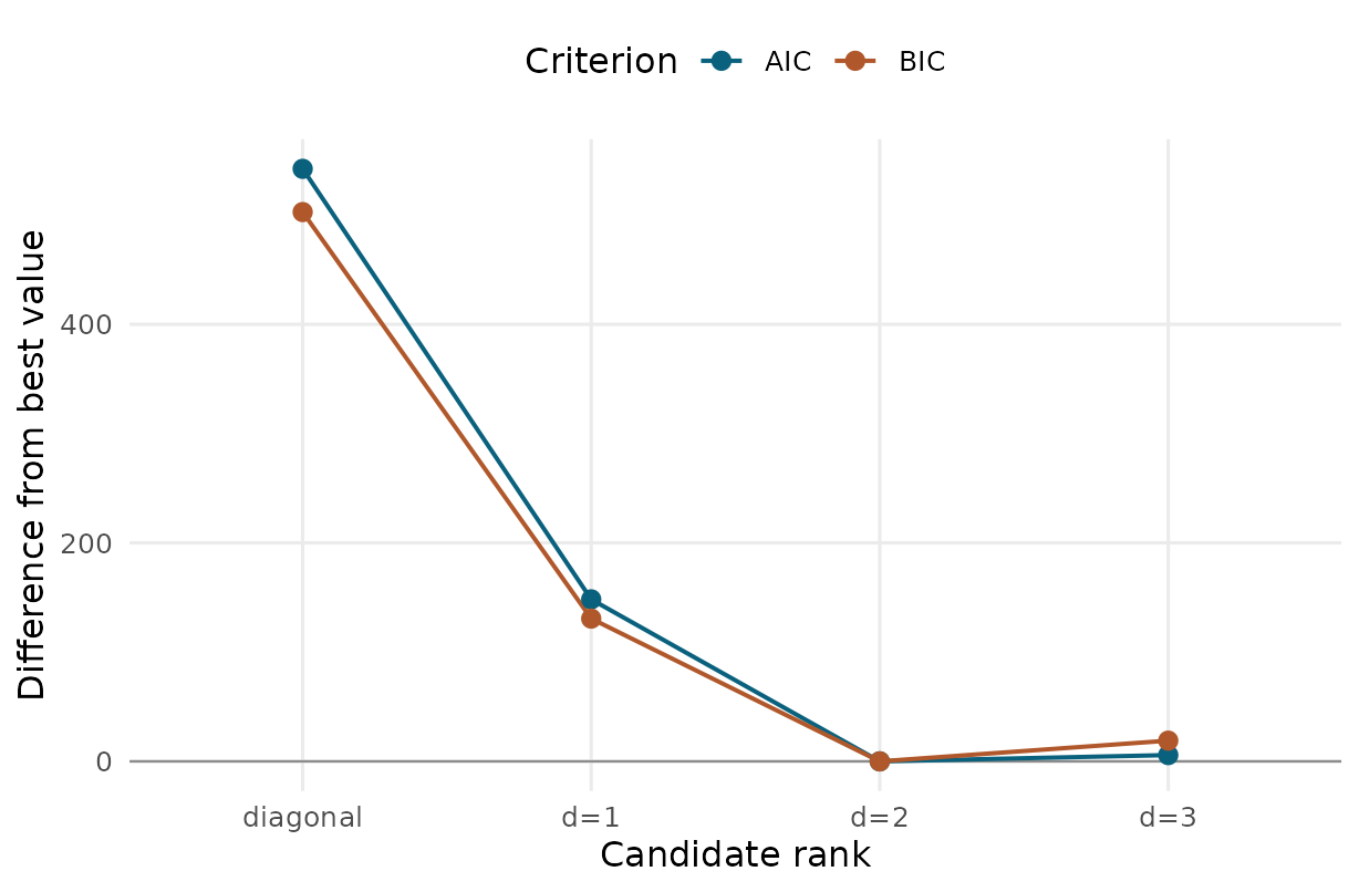
AIC and BIC differences for candidate latent ranks. Both criteria support the planted d = 2 model in this deterministic Gaussian fixture; the overfit d = 3 candidate improves log-likelihood only slightly and is penalised.
Use the criteria as routing information after fit health, not instead of fit health. A model with the lowest AIC/BIC but failed convergence, a non-positive-definite Hessian, or a weak added axis is not ready for biological interpretation.
health_d3 <- check_gllvmTMB(fits$d3)
health_cols <- intersect(
  c("component", "status", "value", "message", "action"),
  names(health_d3)
)
health_d3[
  health_d3$component %in% c(
    "optimizer_convergence",
    "max_gradient",
    "pd_hessian",
    "hessian_rank",
    "weak_axis_unit",
    "cross_loading_structure_unit"
  ),
  health_cols,
  drop = FALSE
]
#>                       component status                                 value
#> 1         optimizer_convergence   PASS                                     0
#> 2                  max_gradient   PASS                             0.0006108
#> 4                    pd_hessian   WARN                                 FALSE
#> 5                  hessian_rank   PASS                                 22/22
#> 11               weak_axis_unit   WARN min=0.0471; shares=0.768,0.0471,0.185
#> 12 cross_loading_structure_unit   PASS                                 0.734
#>                                                        message
#> 1                               optimizer reported convergence
#> 2  largest absolute gradient component at the selected optimum
#> 4      positive-definite Hessian for curvature-based inference
#> 5  rank of the fixed-parameter covariance matrix from sdreport
#> 11              Lambda_B column share of shared loading energy
#> 12      median trait share carried by its dominant latent axis
#>                                                                               action
#> 1       try multiple starts, stronger starts, rescaling, or an alternative optimizer
#> 2               tighten optimization, rescale predictors, or inspect weak components
#> 4   check gradients, boundary variances, rank, starts, and profile/bootstrap targets
#> 5                               treat rank loss as a Hessian/identifiability warning
#> 11 compare lower ranks, inspect fit stability, and avoid over-interpreting weak axes
#> 12 use varimax/promax rotation for interpretation if loadings are spread across axes
If AIC and BIC disagree, treat the disagreement as a prompt to inspect the fitted covariance, weak-axis rows, biological plausibility, and prediction/residual diagnostics. Do not promote a higher rank only because it shaves a small number of AIC units off a numerically weaker fit. Once those checks point to a defensible Gaussian model, use a REML refit only for the final covariance summary, not for the ML candidate table.
Interpret The Selected Model
After choosing a rank, interpret invariant summaries first.
Sigma, correlations, and communalities do not depend on how
the latent variables are rotated. Raw loading columns (obtained with
extract_loadings()) are useful for exploratory labels, but
with d > 1 their signs and rotations need care.
Sigma_hat <- extract_Sigma(fit_selected, level = "unit", part = "total")$Sigma
Sigma_true <- truth$Sigma

ij <- which(upper.tri(Sigma_true, diag = TRUE), arr.ind = TRUE)
sigma_compare <- data.frame(
  entry = paste(rownames(Sigma_true)[ij[, 1]], colnames(Sigma_true)[ij[, 2]],
                sep = " - "),
  type = ifelse(ij[, 1] == ij[, 2], "variance", "covariance"),
  truth = Sigma_true[ij],
  estimate = Sigma_hat[ij],
  stringsAsFactors = FALSE
)

off <- upper.tri(Sigma_true)
data.frame(
  selected_d = selected_d,
  relative_Frobenius_error =
    norm(Sigma_hat - Sigma_true, "F") / norm(Sigma_true, "F"),
  off_diagonal_correlation = stats::cor(Sigma_hat[off], Sigma_true[off])
)
#>   selected_d relative_Frobenius_error off_diagonal_correlation
#> 1          2                0.1260765                0.9841179
lims <- range(c(sigma_compare$truth, sigma_compare$estimate))

ggplot(sigma_compare, aes(truth, estimate, shape = type, colour = type)) +
  geom_abline(slope = 1, intercept = 0, colour = "grey55", linewidth = 0.5) +
  geom_point(size = 2.6, alpha = 0.9) +
  coord_equal(xlim = lims, ylim = lims) +
  scale_colour_manual(values = c(variance = "#0a617d", covariance = "#8c4d8f")) +
  labs(
    x = "True Sigma entry",
    y = "Fitted Sigma entry",
    colour = "Entry",
    shape = "Entry"
  ) +
  theme_minimal(base_size = 12) +
  theme(
    panel.grid.minor = element_blank(),
    legend.position = "top"
  )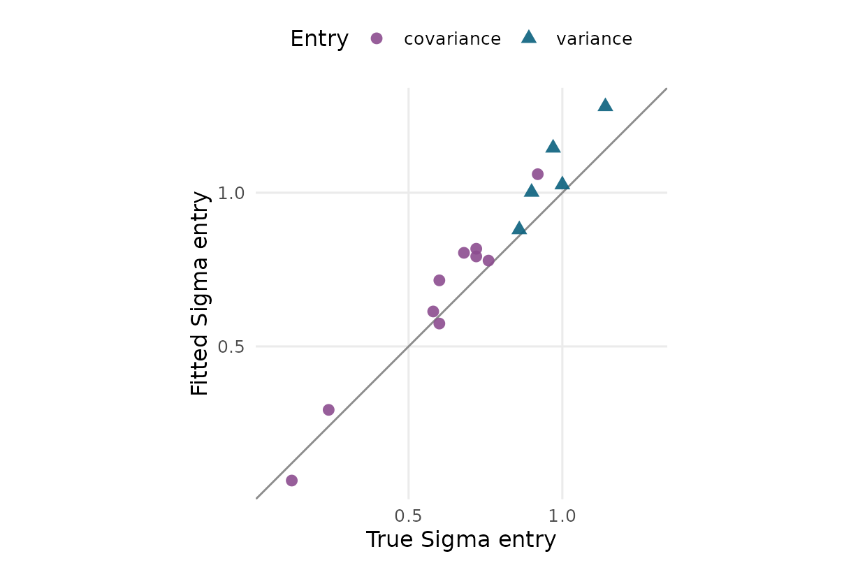
Truth-versus-fit covariance entries for the selected latent-rank model. This rotation-invariant comparison is safer than comparing raw loading columns before rotation or constraints.
The selected rank recovers the planted covariance pattern in this fixture. That statement is narrower than “AIC/BIC proved the true rank.” It means the selected fitted model is a useful summary of this candidate set and this simulated data-generating mechanism. These are recovery numbers on a single deterministic fixture — a display of behaviour on this data-generating mechanism, not empirical coverage across replicate simulations.
Refit The Selected Gaussian Model With REML
The rank comparison above uses maximum likelihood (ML), which is the
estimator used by gllvmTMB() unless
REML = TRUE is supplied. After choosing a Gaussian model to
report, a restricted maximum-likelihood (REML) refit is often the better
variance-component summary because it integrates over the fixed-effect
coefficients before estimating the covariance parameters.
fit_reml_long <- gllvmTMB(
  candidate_formula(selected_d),
  data = df,
  trait = "trait",
  unit = "individual",
  family = gaussian(),
  REML = TRUE,
  control = rank_control
)

fit_reml_wide <- gllvmTMB(
  rank_ex$formula_wide,
  data = df_wide,
  unit = rank_ex$fit_args$unit,
  family = rank_ex$fit_args$family,
  REML = TRUE,
  control = rank_control
)

data.frame(
  estimator = c("ML", "REML"),
  logLik = round(c(
    as.numeric(logLik(fit_selected)),
    as.numeric(logLik(fit_reml_long))
  ), 2),
  df = c(
    attr(logLik(fit_selected), "df"),
    attr(logLik(fit_reml_long), "df")
  ),
  nobs = c(
    attr(logLik(fit_selected), "nobs"),
    attr(logLik(fit_reml_long), "nobs")
  )
)
#>   estimator  logLik df nobs
#> 1        ML -588.18 19  600
#> 2      REML -597.73 19  600

signif(
  abs(as.numeric(logLik(fit_reml_long)) -
        as.numeric(logLik(fit_reml_wide))),
  3
)
#> [1] 0
The ML and REML log-likelihoods answer different questions, so do not
mix them in the AIC/BIC table. Use one estimator consistently for a
candidate set, and report which estimator produced the final covariance
summaries. REML = TRUE is currently guarded to Gaussian
fits without observation weights, retained missing response cells,
mi() predictor models, predictor-informed lv
score means, or Xcoef_fixed maps; its observed fixed-effect
design must also be full rank with positive residual degrees of freedom.
Fixed-effect profile confidence intervals are also ML-only; use Wald
intervals or refit with REML = FALSE before profiling fixed
effects. Both the Wald and profile intervals are nominal, first-order
approximations whose empirical coverage is not yet calibrated for these
models, so treat them as indicative rather than a calibrated decision
rule.
What To Report
Report the candidate set and the checks that constrained it.
| Report item | Why it matters |
|---|---|
| Candidate ranks and formulas | AIC/BIC only compare the models you fit. |
logLik, df, nobs, AIC, BIC,
and deltas |
Readers can see the likelihood gain and the penalty. |
| Estimator for candidate comparison and final covariance summaries | Use one ML candidate table; use REML only for the chosen Gaussian covariance summary. |
check_gllvmTMB() rows |
A low criterion value is not enough when Hessian, gradient, or weak-axis rows warn. |
| Rotation-invariant summaries |
Sigma, correlations, and communalities are safer than
raw loading labels. |
| Biological interpretation | A rank is useful only if the resulting summaries answer the study question. |
This article covers a model-selection workflow for Gaussian ordinary
latent() candidate ranks using base AIC() /
BIC(), logLik(), and
check_gllvmTMB() fit-health rows, then shows a
Gaussian-only REML = TRUE refit for the chosen rank. It
does not validate AIC/BIC as universally correct latent-rank selectors,
calibrate confidence intervals, compare likelihoods from different
fitting approximations, or advertise REML for non-Gaussian, weighted,
retained-missing-response, or mi() predictor fits. It also
does not admit predictor-informed lv score means or
Xcoef_fixed maps under REML. For fitted response
diagnostics, start with Can I trust this
fit?. To evaluate the rank-selection procedure itself, use a
separate target-explicit simulation study with known generating ranks;
simulating only from the selected fitted model cannot answer whether a
lower rank generated the data.