
Temporal covariance for repeated multivariate measurements
Source:vignettes/articles/temporal-ar1.Rmd
temporal-ar1.RmdThis article is for an applied researcher with several traits
measured along an animal, plot, or transect trajectory. Within each
series, the occasions are temporally correlated: time
selects the temporal states, whereas unit and
unit_obs remain ordinary grouping tiers and do not define
the temporal clock. The covariance grammar has five stable-unit sources
and a sixth temporal source for ordered states within a series. This
article teaches the standalone temporal route, with three
trait-covariance modes: temporal_indep(),
temporal_dep(), and rank-one
temporal_latent().
First choose the time scale. AR1 is for ordered integer occasions and preserves their gaps, so . It can describe positive or negative adjacent-occasion persistence. OU is for numeric elapsed time, with positive decay rate and . Translation of elapsed time does not change an OU model; changing its units changes the numerical decay rate. Next choose the trait covariance carried through that time kernel:
| Question about the three traits | Temporal keyword | Trait covariance |
|---|---|---|
| Do they persist separately? | temporal_indep() |
a diagonal variance for each trait |
| May every pair persist together? | temporal_dep() |
an unstructured covariance matrix |
| Is one shared changing axis enough? | temporal_latent(..., d = 1) |
rank-one |
With temporal_latent(unique = TRUE), the model adds its
trait-diagonal
companion, so the temporal covariance is
.
That Psi is correlated through time; it is not independent occasion
noise. Each provider creates a private (series, time) state
index and does not replace the public unit or
unit_obs labels.
This version requires complete Gaussian identity-link data, at least
three traits, and at least three ordered occasions in every series.
Ordinary unit and unit_obs terms can be
combined when their partitions agree and nest. The bounded temporal-only
forecast_temporal(), profile_temporal(),
bootstrap_temporal(), and compare_temporal()
helpers have separate contracts.
Scope boundary. The standalone Gaussian AR1/OU routes shown here have focused local checks for parsing, dense covariance calculations, score labels, simulation, training-data prediction, and update. This is not a general recovery, precision, calibration, or interval-coverage claim. Four narrow replicated AR1 source combinations are also implemented, with separate evidence and restrictions described below. Generic forecasts, new-data prediction, generic profile/bootstrap intervals, and automatic model search or rank selection remain unavailable.
#> Warning: The `label.size` argument of `geom_label()` is deprecated as of ggplot2 3.5.0.
#> ℹ Please use the `linewidth` argument instead.
#> This warning is displayed once per session.
#> Call `lifecycle::last_lifecycle_warnings()` to see where this warning was
#> generated.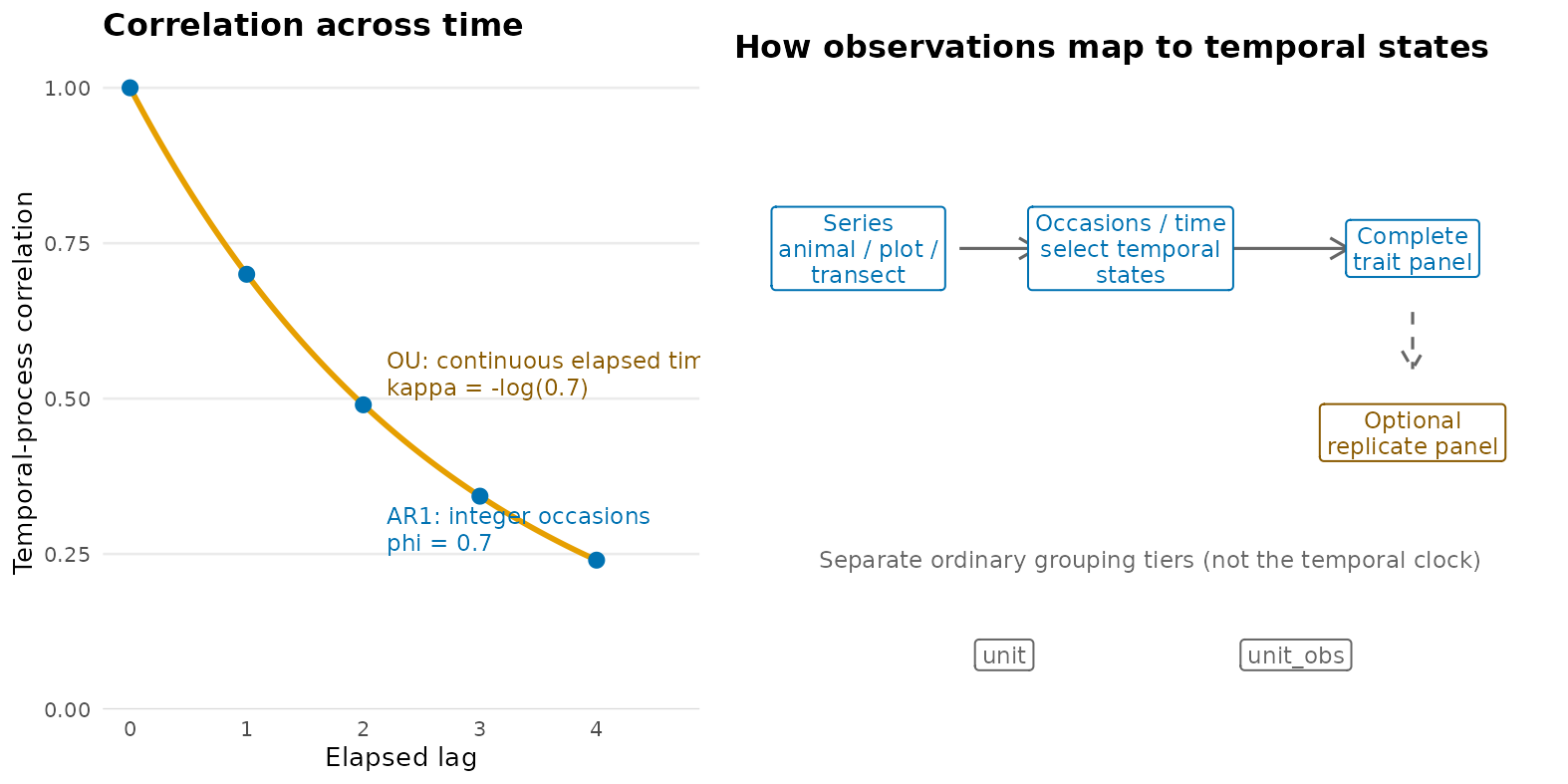
The correlation panel uses fixed illustrative values, not fitted estimates: AR1 has phi = 0.7 and OU has kappa = -log(0.7). The hierarchy panel shows the standalone temporal provider; the restricted additive source combinations described below are not shown.
The AR1 points and OU curve above are conceptual only; they show no fitted estimates and no uncertainty ribbons. With a negative AR1 value, correlations alternate sign across odd and even integer lags. A positive-decay OU process has no analogue of that alternating pattern.
Fit an AR1 model to ordinary longitudinal observations
Here each (series, occasion, trait) cell occurs once.
Start with AR1 because the occasions are integers and their unequal
gaps, 1 to 2 to 4, matter to the covariance. The independent-mode
variance for each trait is its total temporal variance; this
unreplicated design does not split it into occasion and measurement
components.
ordinary <- expand.grid(
  series = paste0("series_", 1:3), occasion = c(1L, 2L, 4L),
  trait = paste0("trait_", 1:3),
  KEEP.OUT.ATTRS = FALSE, stringsAsFactors = FALSE
)
ordinary$value <- rnorm(nrow(ordinary))
The long-format call is canonical. The three fits below differ only
in their cross-trait covariance; extract_temporal() makes
the fitted time index and mode explicit.
fit_long <- gllvmTMB(
  value ~ 0 + trait +
    temporal_indep(0 + trait | series, time = occasion),
  data = ordinary, trait = "trait", unit = "series", family = gaussian(), silent = TRUE
)
Before interpreting the temporal covariance, check the fit. Read and
follow the action for every row that is not
PASS; a converged optimizer alone is not enough. Can I trust this fit? explains the
diagnostic workflow.
health <- check_gllvmTMB(fit_long)
health[health$status != "PASS", c("component", "status", "message", "action")]
#>             component status                             message
#> 11 boundary_sigma_eps   WARN estimated continuous residual scale
#>                                                                                    action
#> 11 if estimated near zero, check row-level unique terms or residual-scale identifiability
extract_temporal(fit_long)
#> $parameters
#>    mode structure     workflow n_series n_pairs
#> 1 indep       ar1 unreplicated        3       9
#>
#> $time
#>   parameter     value
#> 1       phi 0.1839058
#>
#> $pair_index
#>      pair_id   series time
#> 1 series_1.1 series_1    1
#> 4 series_1.2 series_1    2
#> 7 series_1.4 series_1    4
#> 2 series_2.1 series_2    1
#> 5 series_2.2 series_2    2
#> 8 series_2.4 series_2    4
#> 3 series_3.1 series_3    1
#> 6 series_3.2 series_3    2
#> 9 series_3.4 series_3    4
#>
#> $loadings
#> NULL
#>
#> $variance
#>     trait     value               component
#> 1 trait_1 0.1410588 temporal_indep_variance
#> 2 trait_2 0.8204624 temporal_indep_variance
#> 3 trait_3 1.3007920 temporal_indep_variance
fit_dep <- gllvmTMB(
  value ~ 0 + trait + temporal_dep(0 + trait | series, time = occasion),
  data = ordinary, trait = "trait", unit = "series", family = gaussian(), silent = TRUE
)
fit_latent <- gllvmTMB(
  value ~ 0 + trait + temporal_latent(0 + trait | series, time = occasion,
    d = 1, unique = TRUE),
  data = ordinary, trait = "trait", unit = "series", family = gaussian(), silent = TRUE
)
The same observations can be supplied in wide format through the one
gllvmTMB() entry point. traits(...) says which
response columns are the three traits; it expands internally to the same
trait-intercept structure as the long call.
ordinary_wide <- reshape(
  ordinary, idvar = c("series", "occasion"), timevar = "trait",
  direction = "wide"
)
names(ordinary_wide) <- sub("value\\.", "", names(ordinary_wide))
fit_wide <- gllvmTMB(
  traits(trait_1, trait_2, trait_3) ~ 1 +
    temporal_latent(1 | series, time = occasion, d = 1, unique = TRUE),
  data = ordinary_wide, unit = "series", family = gaussian(), silent = TRUE
)
extract_temporal(fit_wide)$pair_index
#>       pair_id   series time
#> 1  series_1.1 series_1    1
#> 10 series_1.2 series_1    2
#> 19 series_1.4 series_1    4
#> 4  series_2.1 series_2    1
#> 13 series_2.2 series_2    2
#> 22 series_2.4 series_2    4
#> 7  series_3.1 series_3    1
#> 16 series_3.2 series_3    2
#> 25 series_3.4 series_3    4
getLV() returns occasion-level scores for
temporal_latent() as a matrix. Its row names and
temporal_index attribute identify the public series and
occasion, rather than the private fitting factor. Score and loading
signs are a reporting convention: the first loading anchors the
displayed direction unless it is negligible relative to the largest
loading, in which case that largest trait anchors it. A simultaneous
sign change leaves the fitted likelihood unchanged.
scores <- getLV(fit_latent)
attr(scores, "temporal_index")
#>      pair_id   series time
#> 1 series_1.1 series_1    1
#> 4 series_1.2 series_1    2
#> 7 series_1.4 series_1    4
#> 2 series_2.1 series_2    1
#> 5 series_2.2 series_2    2
#> 8 series_2.4 series_2    4
#> 3 series_3.1 series_3    1
#> 6 series_3.2 series_3    2
#> 9 series_3.4 series_3    4
predict(fit_latent)
#>      series occasion   trait        est
#> 1  series_1        1 trait_1 -0.2166511
#> 2  series_2        1 trait_1 -0.4150195
#> 3  series_3        1 trait_1 -0.0010643
#> 4  series_1        2 trait_1 -0.2516603
#> 5  series_2        2 trait_1 -0.2783327
#> 6  series_3        2 trait_1  0.2691389
#> 7  series_1        4 trait_1 -0.3479265
#> 8  series_2        4 trait_1 -0.2558673
#> 9  series_3        4 trait_1 -0.2759166
#> 10 series_1        1 trait_2 -1.6843362
#> 11 series_2        1 trait_2  0.5673326
#> 12 series_3        1 trait_2 -0.2047280
#> 13 series_1        2 trait_2 -0.8850913
#> 14 series_2        2 trait_2 -1.2979019
#> 15 series_3        2 trait_2  0.7576684
#> 16 series_1        4 trait_2  0.3661297
#> 17 series_2        4 trait_2  0.1650439
#> 18 series_3        4 trait_2 -0.3465994
#> 19 series_1        1 trait_3  0.1822953
#> 20 series_2        1 trait_3  1.8914775
#> 21 series_3        1 trait_3 -1.0022176
#> 22 series_1        2 trait_3  0.2697428
#> 23 series_2        2 trait_3  1.4030386
#> 24 series_3        2 trait_3 -0.5044382
#> 25 series_1        4 trait_3  1.7873743
#> 26 series_2        4 trait_3 -1.2312050
#> 27 series_3        4 trait_3  1.0927404
Read extract_temporal(fit_latent)$time as the fitted AR1
persistence (or OU decay rate), and use $pair_index to map
each temporal state back to its series and occasion. For the rank-one
model, call
ordination <- extract_ordination(fit_latent, level = "unit"),
then interpret ordination$scores together with
ordination$loadings. This paired accessor applies the same
sign orientation to both: the score traces the shared occasion-level
axis, while each loading gives that trait’s direction and scale on the
axis. Reversing both signs still describes the same fitted model.
Use OU when elapsed time, not occasion number, is meaningful
For elapsed time, use the same grammar with
structure = "ou". Here 0, 0.5, and 2 are elapsed time
points. Do not replace elapsed time with consecutive visit numbers: that
would fit a different scientific model.
ordinary$elapsed <- c(0, 0.5, 2)[match(ordinary$occasion, c(1L, 2L, 4L))]
fit_ou <- gllvmTMB(
  value ~ 0 + trait + temporal_dep(0 + trait | series, time = elapsed,
    structure = "ou"),
  data = ordinary, trait = "trait", unit = "series", family = gaussian(), silent = TRUE
)
extract_temporal(fit_ou)$time
#>   parameter    value
#> 1   ou_rate 2.382545
Add repeated measurements only when they are genuine replicate panels
Use replicate = measurement only when every trait is
measured at least twice at each occasion. It identifies repeated
complete trait panels while the temporal covariance remains on the
series–occasion state. A unit_obs grouping remains an
ordinary, unit-nested random-effect level; it is never silently treated
as a temporal replicate.
replicated <- expand.grid(
  series = paste0("series_", 1:3), occasion = 1:3, measurement = 1:2,
  trait = paste0("trait_", 1:3),
  KEEP.OUT.ATTRS = FALSE, stringsAsFactors = FALSE
)
replicated$value <- rnorm(nrow(replicated))
fit_replicated <- gllvmTMB(
  value ~ 0 + trait + temporal_latent(
    0 + trait | series, time = occasion, replicate = measurement
  ), data = replicated, trait = "trait", unit = "series", family = gaussian(), silent = TRUE
)
extract_temporal(fit_replicated)$variance
#> [1] trait     value     component
#> <0 rows> (or 0-length row.names)
The wide form keeps the measurement column and uses the same keyword.
replicated_wide <- reshape(
  replicated, idvar = c("series", "occasion", "measurement"),
  timevar = "trait", direction = "wide"
)
names(replicated_wide) <- sub("value\\.", "", names(replicated_wide))
fit_replicated_wide <- gllvmTMB(
  traits(trait_1, trait_2, trait_3) ~ 1 + temporal_latent(
    1 | series, time = occasion, replicate = measurement
  ), data = replicated_wide, unit = "series", family = gaussian(), silent = TRUE
)
extract_temporal(fit_replicated_wide)$parameters
#>     mode structure   workflow n_series n_pairs
#> 1 latent       ar1 replicated        3       9
What post-fit actions this standalone route supports
The current post-fit helpers are intentionally limited to an
unreplicated Gaussian temporal_indep() fit.
profile_temporal() re-optimizes the temporal model at fixed
persistence or decay values; bootstrap_temporal() retains
all refit attempts; and compare_temporal() reports AIC
without a likelihood-ratio test. forecast_temporal()
forecasts a complete future trait panel for an already observed series.
Its se.fit is conditional on fitted parameters, not a
calibrated prediction interval.
simulate() redraws stationary temporal scores by
default. Passing condition_on_RE = TRUE keeps the fitted
score modes and redraws only the independent response variation.
update() replays the saved public long or wide call,
rebuilding its private temporal index.
Can I add a phylogeny, pedigree, spatial field, or kernel?
Only four narrow additive combinations are implemented: replicated
AR1 temporal_indep() plus exactly one
kernel_indep(), phylo_indep(),
animal_indep(), or spatial_indep() term. Both
terms describe trait-specific variances, with zero cross-trait
covariance. The model adds their covariance contributions; it does not
fit a source-by-time interaction.
These combinations require complete Gaussian identity-link data,
native TMB/Laplace ML fitting, and at least two complete measurements at
every series–occasion, identified by
replicate = measurement. The source is fixed at
rho = 1. Supply the labelled kernel, tree = or
vcv =, or pedigree =, A =, or
Ainv = inside the corresponding keyword. Use dense
A for a relationship matrix and Ainv for
sparse precision. The spatial route requires a fixed mesh and spatial
contrasts that are not determined solely by temporal lag; spatial range
is still estimated.
For a first exploratory analysis, the kernel combination has
recovered the known pattern in one local simulated example. The
phylogenetic, animal, and spatial combinations have passed focused
likelihood checks, but the recovery studies kept for them were not
accurate enough to support the same conclusion. Treat all four
combinations as exploratory: none has general evidence for recovery,
precision, or interval calibration in other data designs. OU
combinations, temporal dep/latent
combinations, temporal slopes, higher rank, other families, multiple
structured sources, source-by-time interactions, and spatial forecasting
remain unavailable. The temporal-only post-fit helpers above do not
extend to these combinations.
For the standalone examples, inspect the fitted temporal covariance and, for the latent model, report the labelled scores together with the loadings. Read Current limitations before interpreting a more complex model.