Explore loading constraints with suggest_lambda_constraint()

When a reduced-rank model has more than one latent dimension, the columns of its loading matrix $\boldsymbol\Lambda$ can be rotated without changing the shared covariance $\boldsymbol\Lambda\boldsymbol\Lambda^\top$. suggest_lambda_constraint() supplies a reproducible identification scaffold: a matrix that selects one orientation before fitting. It does not discover a biological factor structure or test whether a selected loading is exactly zero.

This page is for an applied user who needs a stable loading orientation for a plot or a reproducible workflow. It uses the binary JSDM teaching fixture, but the point is general. The ecological example below is an orientation demonstration, not evidence for a confirmatory ecological loading structure.

Setup

library(gllvmTMB)
library(ggplot2)

The model and the invariant target

The shipped JSDM fixture records presence or absence for eight species at 120 sites, with a measured environmental predictor. We fit two residual latent dimensions after allowing each species its own environmental response.

jsdm_path <- system.file(
  "extdata", "examples", "joint-sdm-example.rds",
  package = "gllvmTMB"
)
if (!nzchar(jsdm_path)) {
  jsdm_path <- file.path(
    "inst", "extdata", "examples", "joint-sdm-example.rds"
  )
}
jsdm <- readRDS(jsdm_path)
df_long <- jsdm$data_long

For a binomial-logit JSDM, the model is

$$\operatorname{logit}\{P(y_{it}=1)\} = \mathbf{x}_i^\top\boldsymbol\beta_t + \boldsymbol\lambda_t^\top\mathbf{u}_i, \qquad \mathbf{u}_i \sim \mathcal{N}(\mathbf{0}, \mathbf{I}_d).$$

Here $\boldsymbol\lambda_t$ is the row of loadings for species $t$. The individual columns of $\boldsymbol\Lambda$ depend on the chosen orientation; the implied covariance is the more stable scientific target. See Joint species distribution models for a full analysis and Covariance and correlation for the interpretation of $\boldsymbol\Sigma$.

Choose an identification convention before fitting

suggest_lambda_constraint() returns a matrix with NA for an estimated entry and a number for an exact pin. Its default "lower_triangular" convention fixes only the strict upper triangle to zero. For $d = 2$, that is one zero; for $d = K$, it is $K(K - 1)/2$ zeros. These zeros identify an orientation. They are not selected from the JSDM’s fitted loadings.

model_formula <- value ~ 0 + trait + (0 + trait):env_1 +
  latent(0 + trait | site, d = 2)

sug <- suggest_lambda_constraint(
  model_formula,
  data = df_long,
  trait = "trait",
  unit = "site",
  convention = "lower_triangular"
)

sug$constraint
#>      f1 f2
#> sp_1 NA  0
#> sp_2 NA NA
#> sp_3 NA NA
#> sp_4 NA NA
#> sp_5 NA NA
#> sp_6 NA NA
#> sp_7 NA NA
#> sp_8 NA NA
sug$usage_hint
#> [1] "lambda_constraint = list(unit = result$constraint)"

The figure makes the contract visible. The single blue cell is fixed exactly at zero; every white cell is estimated. The first two rows carry the minimal lower-triangular scaffold, while the remaining rows are unconstrained.

constraint_plot <- as.data.frame(as.table(sug$constraint), stringsAsFactors = FALSE)
names(constraint_plot) <- c("species", "dimension", "value")
constraint_plot$status <- ifelse(
  is.na(constraint_plot$value), "estimated", "fixed at 0"
)

ggplot(constraint_plot, aes(x = dimension, y = species, fill = status)) +
  geom_tile(colour = "white", linewidth = 0.7) +
  geom_text(aes(label = ifelse(is.na(value), "estimate", "0")), size = 3) +
  scale_fill_manual(values = c("estimated" = "grey95", "fixed at 0" = "#0A617D")) +
  labs(
    x = "Latent dimension", y = "Species", fill = NULL,
    title = "A lower-triangular loading orientation",
    subtitle = "`NA` means estimate; numeric entries are exact pins"
  ) +
  theme_minimal(base_size = 11) +
  theme(panel.grid = element_blank(), legend.position = "top")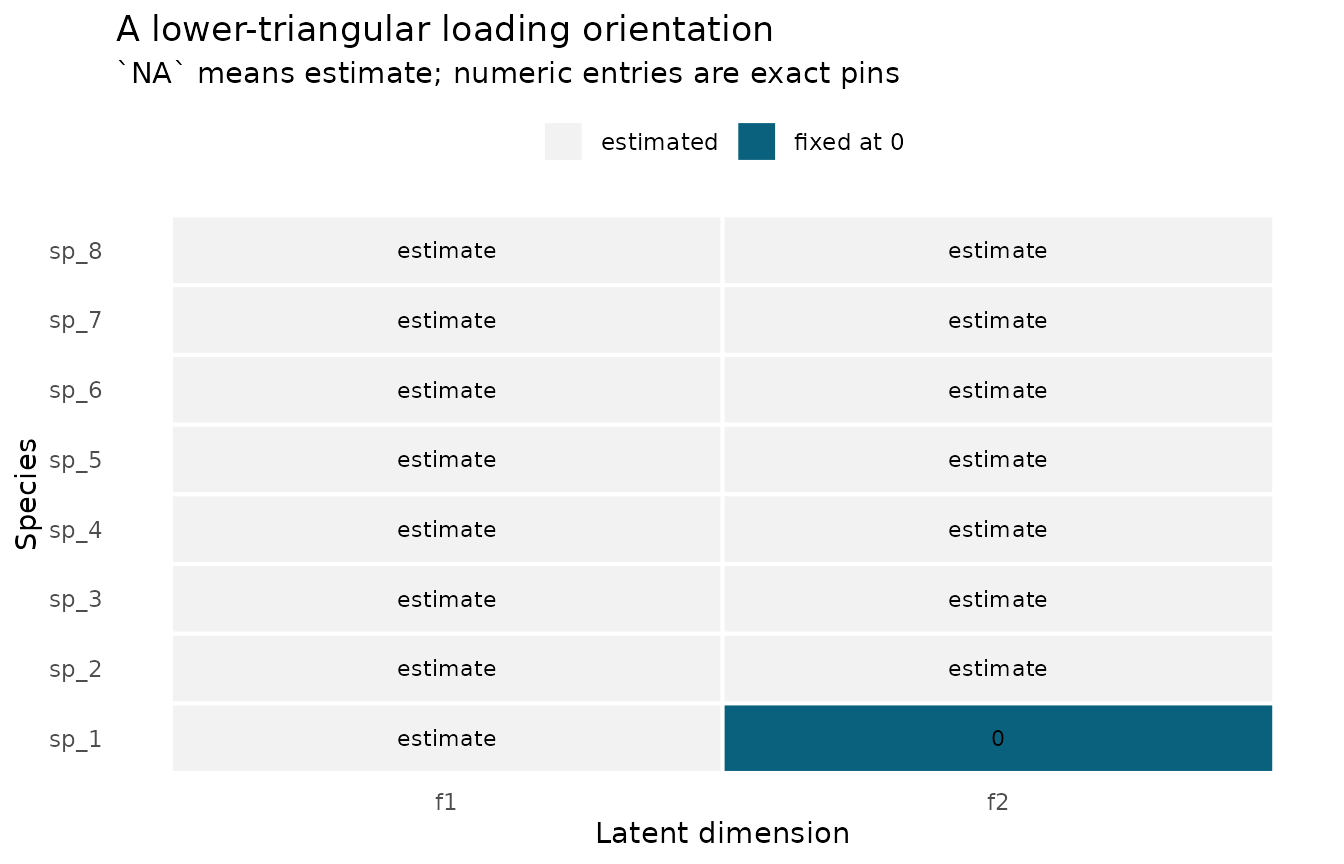

Fit and check the oriented model

Pass the returned matrix to gllvmTMB() through lambda_constraint. The constraint changes the loading orientation, not the purpose of the model: we still interpret residual co-occurrence through $\boldsymbol\Lambda\boldsymbol\Lambda^\top$ and the corresponding latent-scale correlations.

fit_oriented <- gllvmTMB(
  model_formula,
  data = df_long,
  trait = "trait",
  unit = "site",
  family = binomial(),
  lambda_constraint = list(unit = sug$constraint)
)

health <- check_gllvmTMB(fit_oriented)
health[health$component %in% c("optimizer_convergence", "max_gradient", "pd_hessian"), ]
#>               component status     value threshold
#> 1 optimizer_convergence   PASS         0         0
#> 2          max_gradient   PASS 0.0002414      0.01
#> 4            pd_hessian   PASS      TRUE      TRUE
#>                                                       message
#> 1                              optimizer reported convergence
#> 2 largest absolute gradient component at the selected optimum
#> 4     positive-definite Hessian for curvature-based inference
#>                                                                             action
#> 1     try multiple starts, stronger starts, rescaling, or an alternative optimizer
#> 2             tighten optimization, rescale predictors, or inspect weak components
#> 4 check gradients, boundary variances, rank, starts, and profile/bootstrap targets

Do not interpret loading labels if these health rows fail. A constraint can choose a coordinate system; it cannot repair a weakly identified model or add information that the data do not contain.

Sigma_oriented <- extract_Sigma(fit_oriented, level = "unit", part = "shared")
round(Sigma_oriented$Sigma, 2)
#>       sp_1  sp_2  sp_3  sp_4  sp_5  sp_6  sp_7  sp_8
#> sp_1  0.79  0.61  0.57 -0.15 -0.13 -0.46 -0.57 -0.87
#> sp_2  0.61  0.59  0.08 -0.36  0.31 -0.17 -0.65 -0.84
#> sp_3  0.57  0.08  1.57  0.66 -1.39 -0.91  0.24 -0.11
#> sp_4 -0.15 -0.36  0.66  0.55 -0.85 -0.30  0.55  0.52
#> sp_5 -0.13  0.31 -1.39 -0.85  1.48  0.72 -0.65 -0.45
#> sp_6 -0.46 -0.17 -0.91 -0.30  0.72  0.55  0.01  0.24
#> sp_7 -0.57 -0.65  0.24  0.55 -0.65  0.01  0.79  0.93
#> sp_8 -0.87 -0.84 -0.11  0.52 -0.45  0.24  0.93  1.19

Compare exploratory retention conventions

The lower-triangular convention above is fixed before fitting. The other conventions start from an exploratory fit and propose exact zero pins for a new, data-derived constrained refit. They answer different screening questions, so their disagreement is useful to inspect rather than something to hide. Because an exact zero changes the fitted model, its implied covariance can differ from the exploratory fit; this is not merely a coordinate rotation.

fit_exploratory <- gllvmTMB(
  model_formula,
  data = df_long,
  trait = "trait",
  unit = "site",
  family = binomial()
)

comparison_fast <- suggest_lambda_constraints(
  fit_exploratory,
  methods = c("varimax_threshold", "wald_retention"),
  threshold = 0.30,
  retention_prob = 0.90
)
comparison_table <- data.frame(
  convention = c("Varimax threshold", "Wald retention"),
  decision = c(
    "Rotate first, then propose zeros for small standardised loadings.",
    "Propose zeros when the fitted uncertainty does not support a loading above the chosen threshold."
  ),
  proposed_zero_pins = vapply(
    comparison_fast$suggestions,
    function(x) x$n_pins,
    integer(1)
  ),
  free_loadings = vapply(
    comparison_fast$suggestions,
    function(x) length(x$constraint) - x$n_pins,
    integer(1)
  )
)
knitr::kable(comparison_table)

	convention	decision	proposed_zero_pins	free_loadings
varimax_threshold	Varimax threshold	Rotate first, then propose zeros for small standardised loadings.	9	7
wald_retention	Wald retention	Propose zeros when the fitted uncertainty does not support a loading above the chosen threshold.	15	1

varimax_threshold first rotates the loading axes so that species associate more clearly with one dimension. It then standardises each rotated loading as

$$\rho_{tk} = \frac{\Lambda_{tk}}{\sqrt{\Sigma_{\mathrm{total},tt}}}$$

and proposes zero pins when $|\rho_{tk}| < 0.30$. The denominator is the fitted total variance for trait $t$: it includes every latent axis and any fitted diagonal or link-scale variance components. Treat 0.30 as a display choice, not a biological cutoff.

wald_retention uses the same standardised loading. It retains a loading only when the joint delta-method approximation assigns at least 90% probability to its magnitude exceeding 0.30; otherwise it proposes a zero pin. That approximation uses the complete fixed-parameter covariance, including cross-axis covariance and uncertainty in the total-variance denominator. It treats the fitted varimax rotation as fixed, and standardised-loading interval coverage has not been calibrated. Neither convention is a hypothesis test for a biological zero. The figure compares the resulting pin matrices: blue cells are exact zero restrictions in the proposed constrained refit; white cells remain estimated.

make_constraint_frame <- function(suggestion, method) {
  out <- as.data.frame(as.table(suggestion$constraint), stringsAsFactors = FALSE)
  names(out) <- c("species", "dimension", "value")
  out$method <- method
  out$status <- ifelse(is.na(out$value), "estimated", "proposed zero")
  out
}

fast_constraints <- do.call(
  rbind,
  Map(
    make_constraint_frame,
    comparison_fast$suggestions,
    names(comparison_fast$suggestions)
  )
)

ggplot(fast_constraints, aes(x = dimension, y = species, fill = status)) +
  geom_tile(colour = "white", linewidth = 0.7) +
  geom_text(aes(label = ifelse(is.na(value), "estimate", "0")), size = 3) +
  facet_wrap(~ method) +
  scale_fill_manual(values = c("estimated" = "grey95", "proposed zero" = "#0A617D")) +
  labs(
    x = "Latent dimension", y = "Species", fill = NULL,
    title = "Exploratory retention conventions can propose different pins",
    subtitle = "Each blue cell would become an exact zero in a constrained refit"
  ) +
  theme_minimal(base_size = 11) +
  theme(panel.grid = element_blank(), legend.position = "top")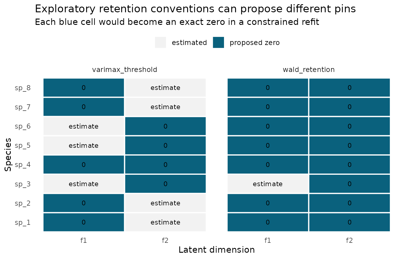

The slower profile-retention convention

profile_retention replaces the Wald screen with a one-entry-at-a-time likelihood-ratio refit. It is useful when you want to see how a likelihood-based screen differs from the fast conventions, but it is not a confirmation procedure: the same exploratory data proposed both the loading and the test. It is also expensive—one refit for each testable loading—and leaves an entry free when a test refit is unhealthy. Run it deliberately after the exploratory fit is healthy.

comparison_profile <- suggest_lambda_constraints(
  fit_exploratory,
  methods = "profile_retention",
  retention_prob = 0.90
)
comparison_profile$suggestions$profile_retention$constraint

# This is a new, data-derived constrained refit, not a harmless rotation of
# the exploratory model. Screen it before describing its covariance summaries.
fit_profile_orientation <- gllvmTMB(
  model_formula,
  data = df_long,
  trait = "trait",
  unit = "site",
  family = binomial(),
  lambda_constraint = list(unit = comparison_profile$recommended$constraint)
)
check_gllvmTMB(fit_profile_orientation)

The code is not run during routine article rendering because it performs many refits. It is intentionally written out in full so that the cost and the post-fit health check are visible rather than hidden. If the exploratory or constrained fit is unhealthy, simplify the model or collect more informative data; do not treat the profile screen as a repair.

What this helper does not establish

The other conventions in suggest_lambda_constraint() include "varimax_threshold", "wald_retention", and "profile_retention". They can propose an exploratory, data-derived constrained refit after inspecting a fit. They do not convert the selected zeros into prior biological hypotheses, and fitting the selected constraint to the same data does not confirm those zeros. Therefore this article does not compare their refits with AIC, BIC, or likelihood-ratio tests, and it does not report loading confidence intervals after selection.

If you have a biological hypothesis before inspecting the data, construct its matrix explicitly with confirmatory_lambda() and state the exact numerical pins as model assumptions. If you need to choose the number of latent dimensions, compare a pre-specified set of candidate ranks with the separate Choosing latent rank workflow. That page uses logLik(), AIC, BIC, and check_gllvmTMB() for its demonstrated Gaussian candidate set; it does not validate information criteria as a universal rank-selection rule.

Next steps

• ?suggest_lambda_constraint documents all conventions and arguments.
• Joint species distribution models shows the full binary occurrence workflow and its rotation-invariant covariance interpretation.
• Can I trust this fit? explains the health table shown above and what to do when a fit is weak.