Behavioural reaction norms with random slopes • gllvmTMB

Evidence boundary. This article demonstrates point estimation for one Gaussian random-slope model. It does not establish calibrated intervals or a general rank-selection procedure for reaction norms.

Repeated measurements can ask two different questions. A behavioural-syndrome model asks whether individuals differ consistently in their average behaviour. A reaction-norm model additionally asks whether individuals differ in their response to a measured context, such as temperature.

This article estimates three kinds of covariance across boldness, exploration, and activity:

covariance among individual intercepts at a declared reference temperature;
covariance among individual temperature slopes; and
covariance between the intercepts and slopes.

Use the simpler behavioural-syndrome model when stable between- and within-individual covariance is the target. Add random slopes only when individual differences in response to a continuous context are scientifically important and each individual has repeated coverage of that context.

Start with the design

library(gllvmTMB)
library(ggplot2)

We use a reproducible simulated example with 60 individuals, five sessions per individual, and three Gaussian response traits. The simulation generator is shipped as data-raw/examples/make-behavioural-reaction-norm-example.R.

rr <- readRDS(system.file(
  "extdata", "examples", "behavioural-reaction-norm-example.rds",
  package = "gllvmTMB"
))
df <- rr$data_long
df_wide <- rr$data_wide
truth <- rr$truth

Temperature is stored both in degrees Celsius and as the centred, scaled predictor used by the model. In a real analysis, save the centring value and scale so that the intercept and slope remain interpretable:

temperature_center_C <- truth$temperature_center_C
temperature_scale_C <- truth$temperature_scale_C

c(
  centre_C = temperature_center_C,
  scale_C = temperature_scale_C
)
#> centre_C  scale_C 
#> 20.01695  5.62833

head(df[c(
  "individual", "session_id", "temperature_C",
  "temperature", "trait", "value"
)], 6)
#>     individual session_id temperature_C temperature       trait      value
#> 1        ind_1    ind_1_1      11.46046   -1.520253    boldness -0.2174060
#> 1.1      ind_1    ind_1_1      11.46046   -1.520253 exploration -0.2267686
#> 1.2      ind_1    ind_1_1      11.46046   -1.520253    activity -0.1589748
#> 2        ind_2    ind_2_1      12.12471   -1.402234    boldness  0.1822026
#> 2.1      ind_2    ind_2_1      12.12471   -1.402234 exploration  0.1212580
#> 2.2      ind_2    ind_2_1      12.12471   -1.402234    activity  0.7823163

Here temperature = 0 means the overall mean temperature. A shift in that origin changes each random intercept from (u) to (u + cb), where (c) is the shift and (b) is the random slope. Intercept variance and intercept–slope covariance therefore depend on the reported reference temperature; slope variance does not.

The essential design check is within-individual coverage. Every simulated individual traverses the planned temperature range, rather than different individuals being observed in different narrow temperature bands:

design <- unique(df_wide[c(
  "individual", "session", "temperature_C", "temperature"
)])
by_individual <- split(design, design$individual)

design_summary <- data.frame(
  quantity = c(
    "minimum sessions per individual",
    "minimum within-individual range (degrees C)",
    "SD of individual mean temperatures (degrees C)"
  ),
  value = c(
    min(vapply(by_individual, nrow, integer(1))),
    min(vapply(
      by_individual,
      function(x) diff(range(x$temperature_C)),
      numeric(1)
    )),
    sd(vapply(
      by_individual,
      function(x) mean(x$temperature_C),
      numeric(1)
    ))
  )
)
knitr::kable(design_summary, digits = 2)

quantity	value
minimum sessions per individual	5.00
minimum within-individual range (degrees C)	14.22
SD of individual mean temperatures (degrees C)	0.26

shown_individuals <- levels(design$individual)[1:12]
ggplot(
  design[design$individual %in% shown_individuals, ],
  aes(session, temperature_C, group = individual)
) +
  geom_line(colour = "#2b6f8a", alpha = 0.55, linewidth = 0.7) +
  geom_point(colour = "#2b6f8a", alpha = 0.75, size = 1.7) +
  scale_x_continuous(breaks = seq_len(truth$n_sessions_per_individual)) +
  labs(
    x = "Session",
    y = "Temperature (degrees C)",
    title = "Repeated context coverage comes before random slopes"
  ) +
  theme_minimal(base_size = 14) +
  theme(panel.grid.minor = element_blank())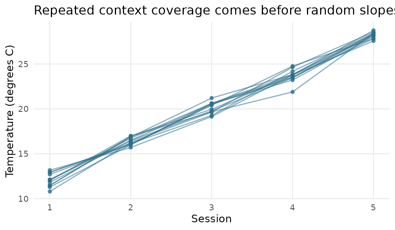

Observed temperatures for 12 example individuals. Every line spans all five sessions and approximately the same temperature range.

If individuals experience systematically different mean environments in an observational study, a single globally centred predictor can mix within-individual response with between-individual exposure differences. In that setting, consider separating the within-individual deviation from the individual’s mean context. Also check confounding with session order, age, season, acclimation, and selective missingness. Without design or experimental support, the fitted temperature slope is an association, not necessarily a causal plastic response.

Long and wide forms of the same model

The long data have one row per (individual, session_id, trait) observation. The wide data have one row per session and one column per response trait:

head(df, 6)
#>     individual session session_id temperature_C temperature       trait
#> 1        ind_1       1    ind_1_1      11.46046   -1.520253    boldness
#> 1.1      ind_1       1    ind_1_1      11.46046   -1.520253 exploration
#> 1.2      ind_1       1    ind_1_1      11.46046   -1.520253    activity
#> 2        ind_2       1    ind_2_1      12.12471   -1.402234    boldness
#> 2.1      ind_2       1    ind_2_1      12.12471   -1.402234 exploration
#> 2.2      ind_2       1    ind_2_1      12.12471   -1.402234    activity
#>          value
#> 1   -0.2174060
#> 1.1 -0.2267686
#> 1.2 -0.1589748
#> 2    0.1822026
#> 2.1  0.1212580
#> 2.2  0.7823163
head(df_wide, 3)
#>   individual session session_id temperature_C temperature   boldness
#> 1      ind_1       1    ind_1_1      11.46046   -1.520253 -0.2174060
#> 2      ind_2       1    ind_2_1      12.12471   -1.402234  0.1822026
#> 3      ind_3       1    ind_3_1      12.69695   -1.300563  0.6345786
#>   exploration   activity
#> 1  -0.2267686 -0.1589748
#> 2   0.1212580  0.7823163
#> 3   0.4534042  0.4418082

The long form makes the trait-specific fixed slopes explicit. The traits(...) form is the equivalent compact syntax for an already-wide data frame:

rr$formula_long
#> value ~ 0 + trait + (0 + trait):temperature + latent(0 + trait + 
#>     (0 + trait):temperature | individual, d = 1) + latent(0 + 
#>     trait | session_id, d = 1)
rr$formula_wide
#> traits(boldness, exploration, activity) ~ 1 + temperature + latent(1 + 
#>     temperature | individual, d = 1) + latent(1 | session_id, 
#>     d = 1)

ctl <- gllvmTMBcontrol(se = TRUE)

fit_long <- gllvmTMB(
  rr$formula_long,
  data = df,
  trait = rr$fit_args$trait,
  unit = rr$fit_args$unit,
  unit_obs = rr$fit_args$unit_obs,
  family = rr$fit_args$family,
  control = ctl
)
#> Warning: ! Ordinary `latent()` now includes a per-trait Psi by default (Sigma = Lambda
#>   Lambda^T + Psi).
#> ℹ This changed in gllvmTMB 0.2.0; earlier `latent()` was loadings-only (Lambda
#>   Lambda^T).
#> → Pass `latent(..., unique = FALSE)` for the old rotation-invariant
#>   loadings-only fit.

fit_wide <- gllvmTMB(
  rr$formula_wide,
  data = df_wide,
  unit = rr$fit_args$unit,
  unit_obs = rr$fit_args$unit_obs,
  family = rr$fit_args$family,
  control = ctl
)

cat(
  "Absolute long/wide log-likelihood difference:",
  signif(abs(as.numeric(logLik(fit_long)) - as.numeric(logLik(fit_wide))), 3),
  "\n"
)
#> Absolute long/wide log-likelihood difference: 0
fit <- fit_long

The individual term contains trait-specific random intercepts and slopes. The session term contains covariance among traits within a repeated occasion:

# Long form
latent(
  0 + trait + (0 + trait):temperature | individual,
  d = 1
)
latent(0 + trait | session_id, d = 1)

# Wide shorthand
latent(1 + temperature | individual, d = 1)
latent(1 | session_id, d = 1)

The simulation plants rank one at each tier, so this example supplies d = 1; it does not select rank one from the data. Use rank sensitivity before interpreting a rank in a new study. We interpret covariance matrices, not named raw latent axes, because an unconstrained loading axis has arbitrary sign and orientation.

Inspect the complete fit health

fit_health <- check_gllvmTMB(fit)
knitr::kable(
  fit_health[c("component", "status", "value")],
  row.names = FALSE
)

component	status	value
optimizer_convergence	PASS	0
max_gradient	PASS	0.0008376
sdreport	PASS	TRUE
pd_hessian	PASS	TRUE
hessian_rank	PASS	24/24
max_fixed_se	PASS	0.07468
restart_history	PASS	1
selected_restart	PASS	1
boundary_flags	PASS	none
rotation_convention_unit_obs	PASS	as_fit_lower_triangular
weak_axis_unit_obs	PASS	min=1; shares=1
near_zero_psi_unit_obs	PASS	0.1073
boundary_sigma_eps	PASS	0.0005998

The audited fixture has optimizer convergence and a raw maximum gradient below 0.01, so its point surface is numerically usable. Standard-error calculations are available, the Hessian is positive definite and full rank, and no boundary flags appear. The final row records that the separate Gaussian residual scale is mapped off. That is expected here because the per-session diagonal Ψ already represents row-level, trait-specific variation. The objective-scaled gradient is descriptive; it is not the convergence cutoff.

Treat warnings according to the quantity they diagnose. An optimizer failure or raw maximum gradient above 0.01 challenges the point covariance and should be repaired before interpretation. An sdreport() or Hessian warning makes local Wald uncertainty unavailable or unreliable, but does not automatically invalidate a stable point covariance; use a supported profile or refit-based bootstrap route when appropriate. A boundary warning requires inspecting the named component and scientific target rather than discarding every summary.

Population-average temperature slopes

The fixed temperature slopes describe the population-average response. They should be inspected before variation among individual slopes:

fixed <- tidy(fit, effects = "fixed")
slope_rows <- grepl(":temperature$", fixed$term)

fixed_slope_table <- data.frame(
  trait = sub(
    ":temperature$",
    "",
    sub("^trait", "", fixed$term[slope_rows])
  ),
  estimate = fixed$estimate[slope_rows],
  SE = fixed$std.error[slope_rows],
  truth = unname(truth$beta),
  per_degree_C = fixed$estimate[slope_rows] / temperature_scale_C
)
knitr::kable(fixed_slope_table, digits = 3)

trait	estimate	SE	truth	per_degree_C
boldness	0.203	0.031	0.18	0.036
exploration	0.087	0.026	0.05	0.015
activity	-0.143	0.018	-0.12	-0.025

In this simulated sample, boldness and exploration increase with temperature, whereas activity decreases. The per-degree column translates the fitted slope back from the standardized predictor. In observational data, describe these as conditional associations unless the design justifies a causal interpretation.

The augmented covariance

For trait (t), individual (i), and session (s), the fitted model is

$y_{ist} = μ_t + β_t x_{is} + u_{it} + b_{it}x_{is} + w_{ist}.$

The individual coefficients are stacked as intercept, slope, intercept, slope, and so on across traits:

$\mathbf a_i = \left(u_{i1}, b_{i1}, u_{i2}, b_{i2}, u_{i3}, b_{i3}\right)^\top, \qquad \mathbf a_i \sim \operatorname{MVN}(0, \Sigma_{B,\mathrm{aug}}).$

The individual covariance is a rank-one shared component plus a diagonal:

$\Sigma_{B,\mathrm{aug}} = \Lambda_{B,\mathrm{aug}}\Lambda_{B,\mathrm{aug}}^\top + \Psi_{B,\mathrm{aug}}.$

At the session tier,

$\mathbf w_{is} \sim \operatorname{MVN}(0, \Sigma_W), \qquad \Sigma_W = \Lambda_W\Lambda_W^\top + \Psi_W.$

The simulation generated a shared session effect plus independent Gaussian noise. With one row per trait and session, those two diagonal sources cannot be estimated separately. The fitted Ψ at the session tier absorbs that noise, so extract_Sigma(level = "unit_obs", part = "total") is the honest total within-session covariance. The model assumes the individual and session effects are independent.

Sigma_shared <- extract_Sigma(
  fit,
  level = "unit_slope",
  part = "shared"
)
Sigma_unique <- extract_Sigma(
  fit,
  level = "unit_slope",
  part = "unique"
)
Sigma_total <- extract_Sigma(
  fit,
  level = "unit_slope",
  part = "total"
)
Sigma_W_total <- extract_Sigma(
  fit,
  level = "unit_obs",
  part = "total"
)

round(Sigma_total$Sigma[intercept_names, intercept_names], 2)
#>                       intercept.boldness intercept.exploration
#> intercept.boldness                  0.32                  0.24
#> intercept.exploration               0.24                  0.25
#> intercept.activity                  0.19                  0.17
#>                       intercept.activity
#> intercept.boldness                  0.19
#> intercept.exploration               0.17
#> intercept.activity                  0.16
round(Sigma_total$Sigma[slope_names, slope_names], 3)
#>                               slope.temperature.boldness
#> slope.temperature.boldness                         0.043
#> slope.temperature.exploration                      0.025
#> slope.temperature.activity                        -0.018
#>                               slope.temperature.exploration
#> slope.temperature.boldness                            0.025
#> slope.temperature.exploration                         0.031
#> slope.temperature.activity                           -0.018
#>                               slope.temperature.activity
#> slope.temperature.boldness                        -0.018
#> slope.temperature.exploration                     -0.018
#> slope.temperature.activity                         0.014
round(Sigma_total$Sigma[intercept_names, slope_names], 3)
#>                       slope.temperature.boldness slope.temperature.exploration
#> intercept.boldness                         0.082                         0.082
#> intercept.exploration                      0.074                         0.073
#> intercept.activity                         0.058                         0.058
#>                       slope.temperature.activity
#> intercept.boldness                        -0.059
#> intercept.exploration                     -0.053
#> intercept.activity                        -0.042

The intercept–intercept block describes stable behavioural covariance at the reference temperature. The slope–slope block describes covariance among individual differences in temperature response. The cross block asks whether individuals above the population mean at the reference temperature tend to have steeper or shallower slopes. That last interpretation changes when the reference temperature changes.

The public extractor also verifies the decomposition:

max(abs(
  Sigma_total$Sigma -
    (Sigma_shared$Sigma + diag(
      Sigma_unique$s,
      nrow = length(Sigma_unique$s)
    ))
))
#> [1] 0

Check recovery block by block

One overall error can hide poor recovery of the smaller slope block. We therefore report each block separately. These are checks of one known simulation, not empirical coverage or a guarantee for other designs.

unit_slope_comparison <- function(estimate, truth) {
  idx <- which(lower.tri(truth, diag = TRUE), arr.ind = TRUE)
  row_name <- rownames(truth)[idx[, "row"]]
  col_name <- colnames(truth)[idx[, "col"]]
  row_is_slope <- grepl("^slope\\.", row_name)
  col_is_slope <- grepl("^slope\\.", col_name)

  data.frame(
    estimate = estimate[idx],
    truth = truth[idx],
    block = ifelse(
      row_is_slope & col_is_slope,
      "slope-slope",
      ifelse(
        !row_is_slope & !col_is_slope,
        "intercept-intercept",
        "intercept-slope"
      )
    )
  )
}

cov_compare <- unit_slope_comparison(
  Sigma_total$Sigma,
  truth$Sigma_unit_slope
)

block_error <- do.call(rbind, lapply(
  split(cov_compare, cov_compare$block),
  function(x) data.frame(
    block = x$block[1],
    mean_absolute_error = mean(abs(x$estimate - x$truth)),
    relative_error = sqrt(sum((x$estimate - x$truth)^2)) /
      sqrt(sum(x$truth^2))
  )
))
knitr::kable(block_error, digits = 3, row.names = FALSE)

block	mean_absolute_error	relative_error
intercept-intercept	0.031	0.127
intercept-slope	0.013	0.174
slope-slope	0.005	0.204

ggplot(cov_compare, aes(truth, estimate, colour = block)) +
  geom_abline(
    slope = 1,
    intercept = 0,
    linetype = 2,
    colour = "grey45"
  ) +
  geom_point(size = 2.6, alpha = 0.88) +
  coord_equal() +
  scale_colour_manual(
    values = c(
      "intercept-intercept" = "#1b9e77",
      "intercept-slope" = "#7570b3",
      "slope-slope" = "#d95f02"
    ),
    name = "Covariance block"
  ) +
  labs(
    x = "Known simulation truth",
    y = "Fitted estimate",
    title = "Recovery by covariance block"
  ) +
  guides(colour = guide_legend(nrow = 2, byrow = TRUE)) +
  theme_minimal(base_size = 14) +
  theme(
    panel.grid.minor = element_blank(),
    legend.position = "bottom"
  )

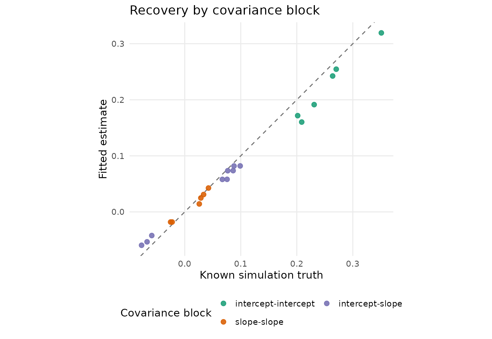
Scatterplot of fitted against known covariance entries. Green points are intercept-intercept entries, purple points are intercept-slope entries, and orange points are slope-slope entries. A dashed diagonal marks exact recovery.

Estimated versus true augmented individual covariance entries. Colours separate the intercept, slope, and cross blocks; the dashed line is perfect recovery.

Pointwise repeatability across temperature

For one trait at standardized temperature (x), the fitted among-individual variance is

$V_{B,t}(x) = \operatorname{Var}(u_{it}) + 2x\operatorname{Cov}(u_{it}, b_{it}) + x^2\operatorname{Var}(b_{it}).$

The pointwise repeatability is

$R_t(x) = \frac{V_{B,t}(x)}{V_{B,t}(x) + (\Sigma_W)_{tt}}.$

This is repeatability at one context value. It is not the correlation between the same individual measured at two different temperatures.

We restrict the curve to the temperature interval observed for every simulated individual. The fitted denominator uses only public covariance output; it does not read an internal residual field.

temperature_support <- split(
  design$temperature,
  design$individual
)
x_grid <- seq(
  max(vapply(temperature_support, min, numeric(1))),
  min(vapply(temperature_support, max, numeric(1))),
  length.out = 80
)

reaction_repeatability <- function(
  Sigma_aug,
  Sigma_W,
  x,
  traits,
  source
) {
  rows <- vector("list", length(traits))
  for (k in seq_along(traits)) {
    trait <- traits[k]
    intercept <- paste0("intercept.", trait)
    slope <- paste0("slope.temperature.", trait)
    between <-
      Sigma_aug[intercept, intercept] +
      2 * x * Sigma_aug[intercept, slope] +
      x^2 * Sigma_aug[slope, slope]
    rows[[k]] <- data.frame(
      trait = trait,
      temperature_C = x * temperature_scale_C + temperature_center_C,
      repeatability = between / (between + Sigma_W[trait, trait]),
      source = source
    )
  }
  do.call(rbind, rows)
}

Sigma_W_truth_total <- truth$Sigma_unit_obs +
  diag(truth$sigma_eps^2, nrow = length(trait_names))
dimnames(Sigma_W_truth_total) <- list(trait_names, trait_names)

repeatability_rows <- rbind(
  reaction_repeatability(
    Sigma_total$Sigma,
    Sigma_W_total$Sigma,
    x_grid,
    trait_names,
    "fitted"
  ),
  reaction_repeatability(
    truth$Sigma_unit_slope,
    Sigma_W_truth_total,
    x_grid,
    trait_names,
    "truth"
  )
)

repeatability_wide <- reshape(
  repeatability_rows,
  idvar = c("trait", "temperature_C"),
  timevar = "source",
  direction = "wide"
)
cat(
  "Mean absolute repeatability error:",
  round(mean(abs(
    repeatability_wide$repeatability.fitted -
      repeatability_wide$repeatability.truth
  )), 3),
  "\n"
)
#> Mean absolute repeatability error: 0.014

ggplot(
  repeatability_rows,
  aes(
    temperature_C,
    repeatability,
    colour = trait,
    linetype = source
  )
) +
  geom_line(linewidth = 0.9) +
  scale_colour_manual(
    values = c(
      boldness = "#1b9e77",
      exploration = "#d95f02",
      activity = "#7570b3"
    ),
    name = "Trait"
  ) +
  scale_linetype_manual(
    values = c(fitted = "solid", truth = "22"),
    name = NULL
  ) +
  scale_y_continuous(
    limits = c(0, 1),
    breaks = seq(0, 1, by = 0.25)
  ) +
  labs(
    x = "Temperature (degrees C)",
    y = "Pointwise repeatability",
    title = "Random slopes make repeatability context-dependent",
    subtitle = "Point estimates within common observed support"
  ) +
  theme_minimal(base_size = 14) +
  theme(
    panel.grid.minor = element_blank(),
    legend.position = "bottom"
  )

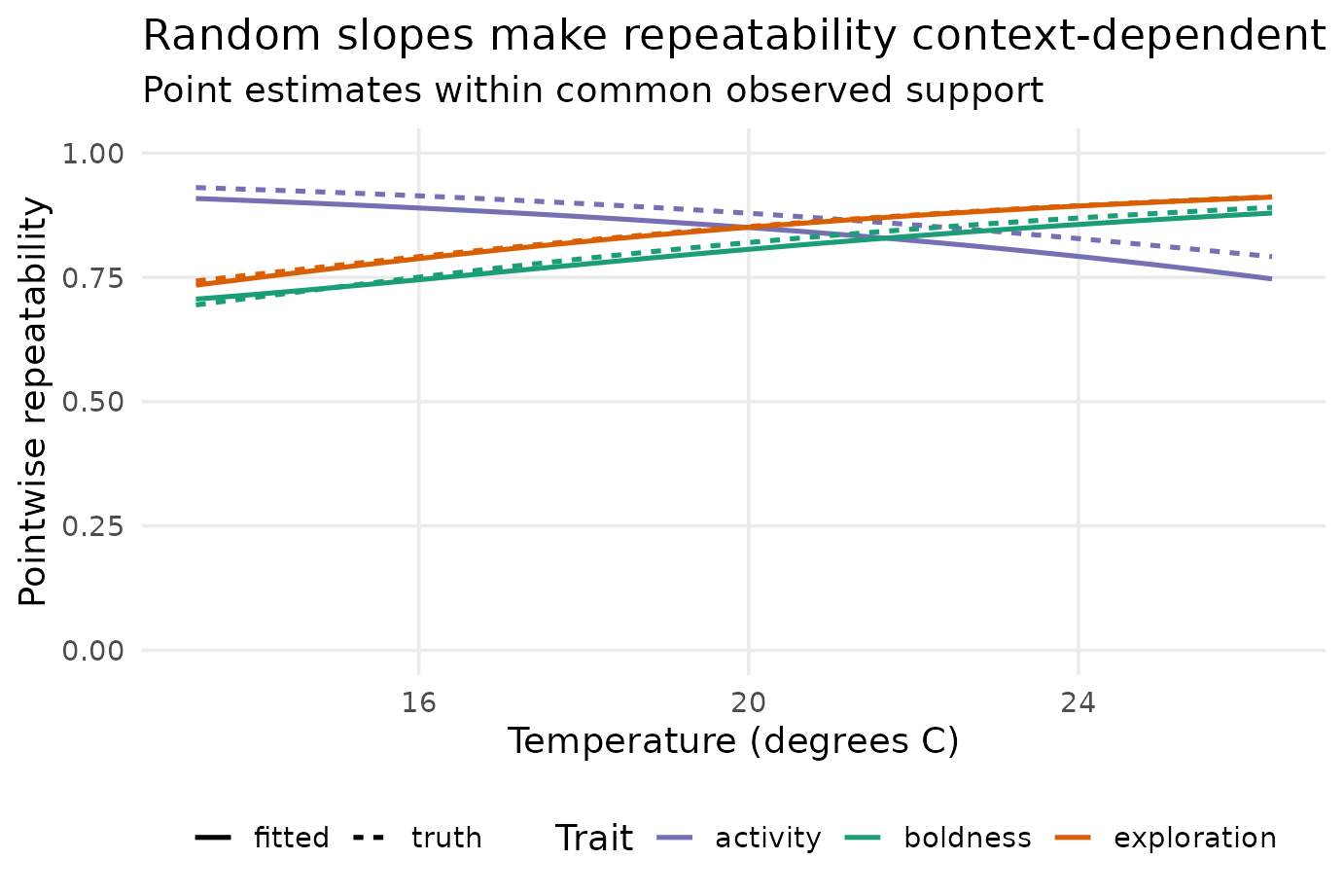
Pointwise repeatability over the temperature interval shared by every simulated individual. Solid lines are fitted point estimates and dashed lines are simulation truth; no uncertainty intervals are claimed.

The curves compare fitted point estimates with one known truth. They do not provide confidence bands or validate interval coverage. In real data, avoid extending the curve beyond well-replicated within-individual support.

What to report

Report the context units, centring value, scaling value, and the actual within-individual context coverage. Then report:

population-average slopes from tidy(fit, effects = "fixed");
the rank supplied at each covariance tier;
the total augmented covariance from extract_Sigma(level = "unit_slope", part = "total");
the reference temperature used to interpret intercept and cross blocks;
the total within-session covariance from extract_Sigma(level = "unit_obs", part = "total"); and
every non-passing row from check_gllvmTMB() before interpreting results.

This worked example is limited to an ordinary Gaussian reaction norm with a rank supplied in advance. It does not establish rank selection, calibrated intervals for variance or repeatability curves, non-Gaussian random-slope inference, or a causal temperature effect. Structured phylogenetic, animal, and spatial random slopes require a separate scientific model and are not evidence for this ordinary individual-level workflow.

Next decision

Interpret the reaction-norm covariance only when individuals cover the environmental gradient, the core health rows pass, and the fitted curve remains inside the observed within-individual range. If the point fit is unhealthy, go to Convergence and hard fits. If the question does not require individual slopes, return to Behavioural syndromes and use the simpler between/within covariance model.

References

Dingemanse, N. J. and Dochtermann, N. A. (2013). Quantifying individual variation in behaviour: mixed-effect modelling approaches. Journal of Animal Ecology 82, 39–54.

O’Dea, R. E., Noble, D. W. A., and Nakagawa, S. (2022). Unifying individual differences in personality, predictability and plasticity: a practical guide. Methods in Ecology and Evolution 13, 278–293.

Stamps, J. A. (2016). Individual differences in behavioural plasticities. Biological Reviews 91, 534–567.