Cross-family trait correlations, including nominal responses

Traits do not arrive on one scale. A single organism carries continuous measurements, presence/absence marks, counts, ordered scores, and unordered categories at once; a single site records abundance, occupancy, and a dominant class. The question this article answers is narrow and concrete: can a Gaussian, a binary, a count, an ordinal, and a nominal trait sit on one shared latent factor in a single gllvmTMB() fit, and can the model report the correlations between those families — including the categorical one?

This page covers only the partially-validated ordinary-unit cross-family route: one multinomial() trait and its non-nominal partners share latent(0 + trait | unit, d). A single powered simulation demonstrates point recovery on that route. It does not admit multiple nominal traits, structured tiers, augmented slopes, or calibrated intervals. The five-family latent covariance is valid, but the one-number observation-scale nominal summary is shown on a non-ordinal subset because the current automatic residual convention is not coherent for an ordinal-probit partner.

Why put different families on one latent scale

The motivation is the same one that drives joint species distribution models and phenotypic-integration analyses: the interesting quantity is not each response on its own but how they covary. If a species that is more abundant is also more likely to be present, and its dominant habitat class shifts with both, that joint structure is the signal. A shared latent factor $\mathbf u_i$ is the device that couples the families: every response loads on the same axes, so a correlation between families is well-defined even though the families live on different observation scales.

The alternative — fit each response separately and correlate the point predictions — discards the measurement model and gives correlations that are biased by each family’s link and dispersion. Putting the families on one latent scale keeps the coupling in the model where it belongs.

The model

For unit $i$ and pseudo-trait $t$ , a $d$ -dimensional shared factor $\mathbf u_i \sim \mathcal N(\mathbf 0, \mathbf I_d)$ drives every family through its own linear predictor and link:

$\eta_{it} = \mu_t + \boldsymbol\lambda_t^{\!\top}\mathbf u_i, \qquad y_{it} \mid \mathbf u_i \sim \text{family}_t(\,g_t^{-1}(\eta_{it})\,).$

Gaussian, binomial, and Poisson traits each occupy a single row of the loading matrix $\boldsymbol\Lambda$ . An ordinal_probit() trait occupies one row and crosses a set of ordered thresholds. A multinomial() trait is different: an unordered response with $K$ categories is not one latent dimension but $K-1$ of them — the baseline-category contrasts — so it expands into $K-1$ rows of $\boldsymbol\Lambda$ , named "<trait>:<cat>". The shared low-rank covariance among all pseudo-traits is $\boldsymbol\Lambda\boldsymbol\Lambda^{\!\top}$ , and the cross-family correlations are its standardised off-diagonals — rotation-invariant, and the quantity to report.

latent() carries a between-unit trait-specific variance $\boldsymbol\Psi$ by default (unique = TRUE), so the full tier covariance is $\boldsymbol\Sigma = \boldsymbol\Lambda\boldsymbol\Lambda^\top + \boldsymbol\Psi$ — $\boldsymbol\Psi$ is the variance each trait has among units beyond the shared factor. For a nominal contrast with one categorical draw per unit, the corresponding between-unit $\boldsymbol\Psi$ is not identified. Replication can identify that variance in principle, but the current engine conservatively maps it off even for the replicated design used here. Admitted partner traits retain their fitted diagonal companion where the model identifies it, so default unique = TRUE still works out of the box; the cross-family correlations assessed below live in $\boldsymbol\Lambda\boldsymbol\Lambda^\top$ .

A five-family worked example

We simulate 500 units, each observed 6 times, with five traits sharing one 3-dimensional factor:

trait	family	value column holds
`g`	`gaussian()`	a real number
`b`	`binomial()`	0 / 1
`p`	`poisson()`	a count
`o`	`ordinal_probit()`	an ordered code `1..Ko`
`cat`	`multinomial()`	a category code `1..K`

The truth is a single loading matrix over the six pseudo-traits g, b, p, o, cat:2, cat:3 (the nominal trait cat contributes the last two rows). Everything the model must recover is contained in $\boldsymbol\Lambda\boldsymbol\Lambda^{\!\top}$ .

library(gllvmTMB)

Simulate

set.seed(20260718)

N     <- 500L   # units
reps  <- 6L     # observations per unit (replication sharpens recovery)
d     <- 3L     # shared latent dimensions
units <- seq_len(N)

# True loadings for the six pseudo-traits on the three shared axes.
# The nominal trait `cat` (K = 3) contributes the rows cat:2 and cat:3.
Lambda <- rbind(
  g       = c( 1.2,  0.2,  0.0),
  b       = c( 0.9,  0.6,  0.1),
  p       = c( 0.3,  1.0,  0.4),
  o       = c( 0.7,  0.4,  0.9),
  `cat:2` = c( 1.0,  0.5,  0.2),
  `cat:3` = c(-0.5,  0.8,  0.6)
)

# Trait means / baseline intercepts (ordinal handled by thresholds instead).
mu  <- c(g = 0, b = 0, p = log(2), o = 0, `cat:2` = 0, `cat:3` = 0)
tau <- c(-1.6, -0.2, 1.2)   # 3 thresholds -> Ko = 4 ordered categories

# One latent position per unit, shared across that unit's replicates.
U   <- matrix(rnorm(N * d), N, d)
Eta <- U %*% t(Lambda)                 # N x 6 unit-level linear predictors
colnames(Eta) <- rownames(Lambda)

sim_one_rep <- function(rep_id) {
  g_val <- mu["g"] + Eta[, "g"] + rnorm(N)                      # Gaussian
  b_val <- rbinom(N, 1L, plogis(mu["b"] + Eta[, "b"]))         # binary
  p_val <- rpois(N, exp(mu["p"] + Eta[, "p"]))                  # count
  o_val <- findInterval(mu["o"] + Eta[, "o"] + rnorm(N), tau) + 1L  # ordinal
  e2 <- mu["cat:2"] + Eta[, "cat:2"]                            # nominal
  e3 <- mu["cat:3"] + Eta[, "cat:3"]                            #   contrasts
  P  <- cbind(1, exp(e2), exp(e3)); P <- P / rowSums(P)         # softmax
  cat_val <- apply(P, 1L, function(pr) sample.int(3L, 1L, prob = pr))
  rbind(
    data.frame(unit = units, trait = "g",   family = "g", value = g_val),
    data.frame(unit = units, trait = "b",   family = "b", value = b_val),
    data.frame(unit = units, trait = "p",   family = "p", value = p_val),
    data.frame(unit = units, trait = "o",   family = "o", value = o_val),
    data.frame(unit = units, trait = "cat", family = "m", value = cat_val)
  )
}

dat <- do.call(rbind, lapply(seq_len(reps), sim_one_rep))
dat$unit   <- factor(dat$unit)
dat$trait  <- factor(dat$trait,  levels = c("g", "b", "p", "o", "cat"))
dat$family <- factor(dat$family, levels = c("g", "b", "p", "o", "m"))

table(dat$trait)
#> 
#>    g    b    p    o  cat 
#> 3000 3000 3000 3000 3000

The family column maps each row to its response family; the nominal trait is the single column cat, whose values are category codes 1..K. It expands into the pseudo-traits cat:2 and cat:3 inside the fit, not in the data.

Fit

One gllvmTMB() call carries all five families on the shared factor. The family argument is a named list keyed by the family column’s levels, and attr(family, "family_var") names that column.

family <- list(
  g = gaussian(), b = binomial(), p = poisson(),
  o = ordinal_probit(), m = multinomial()
)
attr(family, "family_var") <- "family"

fit <- gllvmTMB(
  value ~ 0 + trait + latent(0 + trait | unit, d = 3),  # unique = TRUE (default)
  data   = dat,
  family = family,
  trait  = "trait",
  unit   = "unit",
  silent = TRUE
)

c(convergence = fit$opt$convergence, pdHess = isTRUE(fit$sd_report$pdHess))
#> convergence      pdHess 
#>           0           1

Recover the cross-family correlations

extract_Sigma() with part = "shared" returns the latent low-rank covariance $\boldsymbol\Lambda\boldsymbol\Lambda^{\!\top}$ over all six pseudo-traits. We standardise it and compare against the truth built from Lambda.

Sigma_true <- Lambda %*% t(Lambda)
R_true <- cov2cor(Sigma_true)

Sig_hat <- extract_Sigma(fit, level = "unit", part = "shared", link_residual = "none")
R_hat   <- cov2cor(Sig_hat$Sigma)

# align the recovered matrix to the truth's ordering by name
ord   <- rownames(R_true)
R_hat <- R_hat[ord, ord]

pairs <- rbind(
  c("g", "b"), c("g", "p"), c("g", "o"),
  c("g", "cat:2"), c("g", "cat:3"),
  c("b", "cat:2"), c("p", "cat:3"), c("o", "cat:2")
)

data.frame(
  pair      = paste(pairs[, 1], pairs[, 2], sep = " ~ "),
  true      = round(mapply(function(i, j) R_true[i, j], pairs[, 1], pairs[, 2]), 3),
  recovered = round(mapply(function(i, j) R_hat[i, j], pairs[, 1], pairs[, 2]), 3),
  row.names = NULL
)
#>        pair   true recovered
#> 1     g ~ b  0.908     0.857
#> 2     g ~ p  0.412     0.431
#> 3     g ~ o  0.626     0.644
#> 4 g ~ cat:2  0.941     0.927
#> 5 g ~ cat:3 -0.323    -0.254
#> 6 b ~ cat:2  0.989     0.972
#> 7 p ~ cat:3  0.712     0.756
#> 8 o ~ cat:2  0.787     0.824

The recovered correlations track the truth across all five families, including the two nominal contrasts cat:2 and cat:3 and their sign — a strong positive g ~ cat:2, a negative g ~ cat:3. The remaining error is sampling noise at this N; larger N (or more replicates per unit) shrinks it. Every off-diagonal pair, not just the eight highlighted here, is available in R_hat.

offd <- upper.tri(R_true)
plot(R_true[offd], R_hat[offd],
     xlab = "true correlation", ylab = "recovered correlation",
     xlim = c(-1, 1), ylim = c(-1, 1), pch = 19, col = "#3366aa")
abline(0, 1, lty = 2, col = "grey40")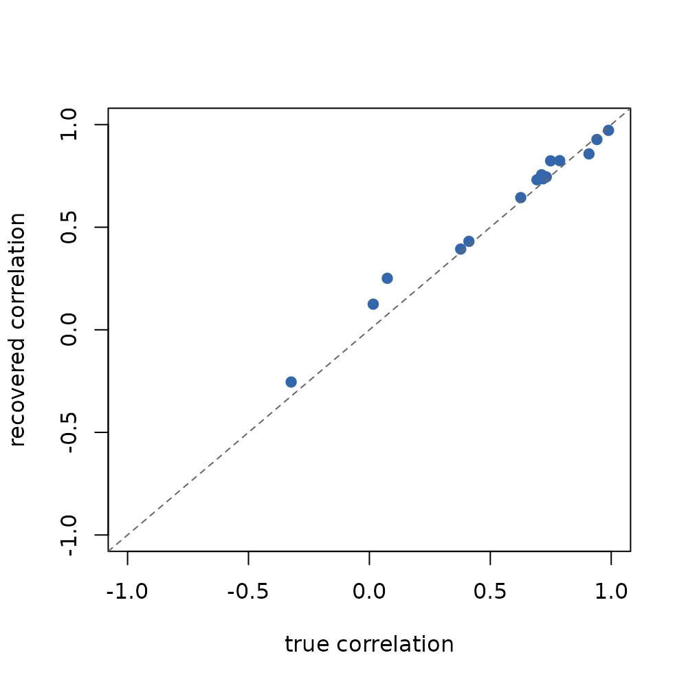

True versus recovered latent cross-family correlations, all off-diagonal pairs. The line is the identity; points near it indicate faithful recovery in this powered run.

Summarising the nominal trait: the 2C multiple correlation

The pairwise table above lists a separate correlation for each nominal contrast (cat:2, cat:3). Often a reader wants one number for “how strongly is the categorical trait associated with each partner?” that does not depend on which category was chosen as the reference. That is what extract_cross_correlations() reports (reporting decision 2C): a reference-invariant multiple correlation between the categorical trait and each single-scale partner, optionally with the underlying $(K-1)$ -vector.

The five-family fit contains an ordinal-probit partner. Its threshold model already fixes the latent residual at one, so an "auto" summary would add that unit residual a second time. extract_cross_correlations() therefore refuses that combination rather than attenuating the reported association. We retain the valid five-family latent-covariance result above, then refit the same data without the ordinal trait for the observation-scale one-number summary.

ordinal_refusal <- tryCatch(
  extract_cross_correlations(fit, level = "unit", link_residual = "auto"),
  error = conditionMessage
)
ordinal_refusal
#> [1] "\033[1m\033[22mThe observation-scale nominal summary is unavailable with an\nordinal-probit partner.\n\033[36mℹ\033[39m Ordinal-probit partner traits: o.\n\033[36mℹ\033[39m The threshold model already fixes each ordinal latent residual at 1;\n  `link_residual = \"auto\"` would add it again.\n→ Use a supported non-ordinal partner set for `extract_cross_correlations()`,\n  or report latent-scale pairwise quantities with `extract_Sigma(..., part =\n  \"shared\", link_residual = \"none\")`."

dat_summary <- droplevels(dat[dat$trait != "o", ])
family_summary <- family[c("g", "b", "p", "m")]
attr(family_summary, "family_var") <- "family"

fit_summary <- gllvmTMB(
  value ~ 0 + trait + latent(0 + trait | unit, d = 3),
  data   = dat_summary,
  family = family_summary,
  trait  = "trait",
  unit   = "unit",
  silent = TRUE
)

xc <- extract_cross_correlations(
  fit_summary, level = "unit", link_residual = "auto"
)
xc
#>   nominal partner multiple_r
#> 1     cat       g  0.6314987
#> 2     cat       b  0.3014727
#> 3     cat       p  0.4188391

The single-number summary is reported on the observation scale. The "auto" route adds the applicable family-specific residual for each admitted partner and the full softmax residual matrix for the nominal block. This is the deliberate default, and the reason is in the next section.

Honest caveats

These are limits of the capability as it stands at 0.6, not incidental notes.

Fitted $\boldsymbol\Psi$ and the fixed link residual are different objects. The between-unit $\boldsymbol\Psi$ inside latent() is an estimated among-unit diagonal companion. The extractor’s $R_{\mathrm{link}}$ is a separate family-specific observation-scale addition; for the nominal block it is $(\pi^2/6)(\mathbf I+\mathbf J)$ . With one categorical draw per unit the nominal contrast $\boldsymbol\Psi$ is not identified. Replication can identify it in principle, but the current engine conservatively maps it off even in the replicated design here; admitted partner diagonals remain fitted where the model identifies them. A replication-aware multinomial refinement is future work. Either way the pairwise latent correlations (the matrix) are the recovered quantities. See the vocabulary of $\boldsymbol\Psi$ and covariance and correlation.
The single-number summary belongs on the observation scale. For an admitted non-ordinal partner set, the reference-invariant multiple correlation uses each applicable family-specific residual and the softmax residual $(\pi^2/6)(\mathbf I + \mathbf J)$ — the covariance of the differenced Gumbel errors in the random-utility representation of the softmax (McFadden 1974), which reduces to the binomial’s $\pi^2/3$ when $K = 2$ . On the latent scale (link_residual = "none") the multiple correlation degenerates toward 1 whenever the $K-1$ contrast block spans the partner, because a $(K-1)$ -dimensional block can align with almost any single direction. That is why the observation scale is the sensible default for the one-number summary, while the per-pair latent correlations remain the right object for the matrix. Ordinal-probit is not admitted on this automatic summary route because its residual is already fixed by the threshold model; the typed refusal above prevents double counting.
Recovering a nominal trait’s covariance is data-hungry. A single categorical draw carries little information about a $(K-1)$ -dimensional liability. With one draw per unit the reduced-rank estimate can rail at $\pm 1$ ; this is an information limitation, not a bug. It resolves with replication (multiple draws per unit, as here) or many units. The powered regime in this article — 500 units $\times$ 6 replicates — is what makes the recovery above possible; do not expect the same at one observation per unit.
Intervals are not yet calibrated. This is a 0.6 capability. Coverage of the cross-family correlations has not been certified; treat the recovered numbers and any interval outputs as recovery-oriented, not as calibrated confidence statements.
One multinomial trait per fit. The current implementation supports a single multinomial() trait in a fit. Two nominal responses on one shared factor is not yet supported.