
Where does the tree go?
Source:vignettes/articles/where-does-the-tree-go.Rmd
where-does-the-tree-go.RmdThe tree belongs to the axis it explains
A phylogeny supplies covariance for species labels on a particular model axis. It does not replace the other covariance sources in the scientific model. Here species are the rows of a morphology matrix, but the columns of a community matrix. Both examples use synthetic Gaussian responses.
These examples separate tree-structured covariance from ordinary residual covariance. They illustrate one synthetic realization; they do not establish parameter recovery or interval coverage.
library(gllvmTMB)
#> gllvmTMB is experimental. Use a documented tutorial, inspect fit diagnostics, and read Current limitations and boundaries before treating an estimate or interval as a scientific result. Convergence alone is not enough.
library(ape)
library(ggplot2)

# Use the same deterministic first start for each displayed fit.
fit_control <- gllvmTMBcontrol(
  se = FALSE, n_init = 1L, optimizer = "nlminb", optArgs = list(),
  init_jitter = 0, start_method = list(method = NULL, jitter.sd = 0)
)
Simulation helpers: run this code once before the examples
The code below fixes the trees, predictors, loading matrices and diagonal variances before fitting. It generates one realization, not a recovery study.
## Synthetic data construction; all seeds and covariance parameters are fixed.

TREE_AXIS_FIXTURE_VERSION <- "tree-axis-latent-v1"
TREE_AXIS_SEEDS <- list(
  morphology_tree = 202608301L,
  morphology_phy = 202608302L,
  morphology_non = 202608303L,
  morphology_elevation = 202608304L,
  community_tree = 202608401L,
  community_latitude = 202608402L,
  community_coef = 202608403L,
  community_site = 202608404L
)

.tree_axis_unit_height <- function(tree) {
  height <- max(ape::node.depth.edgelength(tree))
  if (!is.finite(height) || height <= 0) stop("Tree height must be positive.")
  tree$edge.length <- tree$edge.length / height
  tree
}

.tree_axis_tree_covariance <- function(tree, labels) {
  tip_heights <- ape::node.depth.edgelength(tree)[seq_along(tree$tip.label)]
  if (max(abs(tip_heights - 1)) > 1e-10) {
    stop("The frozen tree must be ultrametric with unit tip height.")
  }
  K <- ape::vcv.phylo(tree, corr = TRUE)[labels, labels, drop = FALSE]
  K_unit_height <- ape::vcv.phylo(tree, corr = FALSE)[labels, labels, drop = FALSE]
  if (max(abs(K - K_unit_height)) > 1e-8) {
    stop("Tree covariance changed scale after unit-height normalization.")
  }
  K
}

.tree_axis_draw_source <- function(K, Lambda, Psi, seed) {
  set.seed(seed)
  n <- nrow(K)
  p <- nrow(Lambda)
  L_K <- t(chol(K))
  shared <- L_K %*% matrix(rnorm(n * ncol(Lambda)), n, ncol(Lambda)) %*%
    t(Lambda)
  unique <- L_K %*% matrix(rnorm(n * p), n, p) %*% chol(Psi)
  list(shared = shared, unique = unique, total = shared + unique)
}

.tree_axis_draw_iid <- function(n, Lambda, Psi, seed) {
  set.seed(seed)
  p <- nrow(Lambda)
  shared <- matrix(rnorm(n * ncol(Lambda)), n, ncol(Lambda)) %*% t(Lambda)
  unique <- matrix(rnorm(n * p), n, p) %*% chol(Psi)
  list(shared = shared, unique = unique, total = shared + unique)
}

.tree_axis_morphology <- function(size = c("target", "canary")) {
  size <- match.arg(size)
  set.seed(TREE_AXIS_SEEDS$morphology_tree)
  n_species <- if (identical(size, "target")) 80L else 20L
  species <- sprintf("morph_%03d", seq_len(n_species))
  traits <- c(
    "leaf_area", "specific_leaf_area", "leaf_dry_matter",
    "stem_height", "seed_mass", "root_depth"
  )
  tree <- .tree_axis_unit_height(ape::rcoal(n_species))
  tree$tip.label <- species
  K <- .tree_axis_tree_covariance(tree, species)

  ## Two deliberately non-collinear trait contrasts.  Their signs label a
  ## synthetic fixture; they do not assert mechanisms in real plants.
  Lambda_phy <- matrix(c(
    0.62, 0.10,
    0.48, 0.34,
   -0.18, 0.58,
    0.71,-0.08,
    0.10, 0.64,
    0.42,-0.38
  ), nrow = length(traits), byrow = TRUE,
  dimnames = list(traits, c("leaf_stature", "reproductive_structure")))
  Lambda_non <- matrix(c(
    0.22, 0.46,
    0.54,-0.16,
    0.63, 0.28,
   -0.15, 0.52,
    0.48,-0.24,
    0.08, 0.57
  ), nrow = length(traits), byrow = TRUE,
  dimnames = list(traits, c("resource_axis", "independent_axis")))
  psi_phy <- c(0.20, 0.16, 0.24, 0.18, 0.22, 0.14)
  psi_non <- c(0.18, 0.25, 0.17, 0.21, 0.15, 0.23)
  Psi_phy <- diag(psi_phy)
  Psi_non <- diag(psi_non)
  dimnames(Psi_phy) <- dimnames(Psi_non) <- list(traits, traits)

  phy <- .tree_axis_draw_source(K, Lambda_phy, Psi_phy, TREE_AXIS_SEEDS$morphology_phy)
  non <- .tree_axis_draw_iid(n_species, Lambda_non, Psi_non,
                              TREE_AXIS_SEEDS$morphology_non)
  set.seed(TREE_AXIS_SEEDS$morphology_elevation)
  elevation <- as.numeric(scale(seq(-1.6, 1.6, length.out = n_species) +
    rnorm(n_species, sd = 0.20)))
  trait_intercept <- c(0.25, 0.05, -0.15, 0.40, -0.25, 0.10)
  trait_elevation <- c(0.20, 0.32, -0.18, 0.38, -0.10, 0.14)
  Y <- sweep(phy$total + non$total, 2L, trait_intercept, "+") +
    tcrossprod(elevation, trait_elevation)
  colnames(Y) <- traits

  wide <- data.frame(species = factor(species, levels = species), elevation = elevation,
                     check.names = FALSE)
  wide[traits] <- as.data.frame(Y, check.names = FALSE)
  long <- data.frame(
    species = factor(rep(species, each = length(traits)), levels = species),
    elevation = rep(elevation, each = length(traits)),
    trait = factor(rep(traits, times = n_species), levels = traits),
    value = as.vector(t(Y))
  )
  list(
    species = species, traits = traits, tree = tree, K = K, long = long, wide = wide,
    truth = list(
      Lambda_phy = Lambda_phy, Psi_phy = Psi_phy,
      Sigma_phy_shared = tcrossprod(Lambda_phy),
      Sigma_phy_total = tcrossprod(Lambda_phy) + Psi_phy,
      Lambda_non = Lambda_non, Psi_non = Psi_non,
      Sigma_non_shared = tcrossprod(Lambda_non),
      Sigma_non_total = tcrossprod(Lambda_non) + Psi_non,
      elevation = trait_elevation
    )
  )
}

.tree_axis_community <- function(size = c("target", "canary")) {
  size <- match.arg(size)
  n_sites <- if (identical(size, "target")) 150L else 50L
  n_species <- if (identical(size, "target")) 50L else 20L
  species <- sprintf("plant_%03d", seq_len(n_species))
  set.seed(TREE_AXIS_SEEDS$community_latitude)
  sites <- data.frame(
    site_id = sprintf("site_%03d", seq_len(n_sites)),
    latitude = as.numeric(scale(seq(38, 62, length.out = n_sites) +
      rnorm(n_sites, sd = 0.7)))
  )
  set.seed(TREE_AXIS_SEEDS$community_tree)
  tree <- .tree_axis_unit_height(ape::rcoal(n_species))
  tree$tip.label <- species
  K <- .tree_axis_tree_covariance(tree, species)
  pathway <- factor(rep(c("C3", "C4"), length.out = n_species), levels = c("C3", "C4"))
  column_data <- data.frame(trait = species, pathway = pathway)

  pathway_intercept <- c(C3 = 0.85, C4 = 0.45)
  pathway_slope <- c(C3 = -0.30, C4 = 0.55)
  rho_truth <- 0.60
  K_rho <- rho_truth * K + (1 - rho_truth) * diag(diag(K))
  coefficient_sd <- c(`(Intercept)` = 0.18, latitude = 0.55)
  coefficient_cor <- -0.25
  Sigma_coef <- outer(coefficient_sd, coefficient_sd) *
    matrix(c(1, coefficient_cor, coefficient_cor, 1), 2L,
           dimnames = list(names(coefficient_sd), names(coefficient_sd)))
  set.seed(TREE_AXIS_SEEDS$community_coef)
  coefficient_draw <- t(chol(K_rho)) %*%
    matrix(rnorm(n_species * 2L), n_species, 2L) %*% chol(Sigma_coef)
  colnames(coefficient_draw) <- names(coefficient_sd)
  rownames(coefficient_draw) <- species

  ## Conditional residual association across species at a site.  There is no
  ## fifth Gaussian noise term: Psi_site is the cell-level independent part.
  Lambda_site <- cbind(
    0.48 * (sin(seq_len(n_species) * 0.22) + 0.20),
    -0.32 * (cos(seq_len(n_species) * 0.31) - 0.15)
  )
  rownames(Lambda_site) <- species
  colnames(Lambda_site) <- c("cooccurrence_axis_1", "cooccurrence_axis_2")
  psi_site <- seq(0.12, 0.28, length.out = n_species)
  Psi_site <- diag(psi_site)
  dimnames(Psi_site) <- list(species, species)
  residual <- .tree_axis_draw_iid(n_sites, Lambda_site, Psi_site,
                                   TREE_AXIS_SEEDS$community_site)$total
  alpha <- pathway_intercept[as.character(pathway)] + coefficient_draw[, "(Intercept)"]
  beta <- pathway_slope[as.character(pathway)] + coefficient_draw[, "latitude"]
  Y <- outer(rep(1, n_sites), alpha) + tcrossprod(sites$latitude, beta) + residual
  colnames(Y) <- species

  wide <- data.frame(site_id = sites$site_id, latitude = sites$latitude,
                     check.names = FALSE)
  wide[species] <- as.data.frame(Y, check.names = FALSE)
  long <- data.frame(
    site_id = factor(rep(sites$site_id, each = n_species), levels = sites$site_id),
    latitude = rep(sites$latitude, each = n_species),
    trait = factor(rep(species, times = n_sites), levels = species),
    pathway = factor(rep(as.character(pathway), times = n_sites), levels = c("C3", "C4")),
    value = as.vector(t(Y))
  )
  list(
    species = species, sites = sites, tree = tree, K = K,
    long = long, wide = wide, column_data = column_data,
    truth = list(
      pathway_intercept = pathway_intercept, pathway_slope = pathway_slope,
      rho = rho_truth, K_rho = K_rho, Sigma_coef = Sigma_coef,
      coefficient_draw = coefficient_draw, Lambda_site = Lambda_site,
      Psi_site = Psi_site, Sigma_site_shared = tcrossprod(Lambda_site),
      Sigma_site_total = tcrossprod(Lambda_site) + Psi_site
    )
  )
}

make_tree_axis_fixture <- function(size = c("target", "canary")) {
  size <- match.arg(size)
  out <- list(
    version = TREE_AXIS_FIXTURE_VERSION,
    morphology = .tree_axis_morphology(size),
    community = .tree_axis_community(size)
  )
  stopifnot(
    identical(levels(out$morphology$long$species), out$morphology$tree$tip.label),
    identical(levels(out$community$long$trait), out$community$tree$tip.label),
    nrow(out$morphology$long) == length(out$morphology$species) * length(out$morphology$traits),
    nrow(out$community$long) == nrow(out$community$sites) * length(out$community$species),
    qr(out$community$truth$Lambda_site)$rank == 2L
  )
  out
}
corplot <- function(S, title) {
  z <- as.data.frame(as.table(stats::cov2cor(S)))
  names(z) <- c("first", "second", "r")
  p <- ggplot(z, aes(first, second, fill = r)) +
    geom_tile(colour = "white", linewidth = 0.15) +
    scale_fill_gradient2(low = "#b2182b", mid = "white", high = "#2166ac",
                         limits = c(-1, 1)) +
    coord_equal() + labs(title = title, x = NULL, y = NULL, fill = "Correlation") +
    theme_minimal(base_size = 10) +
    theme(axis.text.x = element_text(angle = 45, hjust = 1),
          plot.title = element_text(size = 11, face = "bold"),
          panel.grid = element_blank())
  if (nrow(S) <= 12) {
    p <- p + geom_text(aes(label = sprintf("%.2f", r)), size = 2.6)
  } else {
    keep <- rownames(S)[unique(c(1L, seq(10L, nrow(S), by = 10L)))]
    p <- p + scale_x_discrete(breaks = keep) + scale_y_discrete(breaks = keep)
  }
  p
}
axes <- data.frame(
  example = c("1. Species × traits", "2. Sites × species"),
  rows = c("Species rows: tree A", "Site rows: ordinary latent()"),
  columns = c("Trait columns", "Species columns: tree K for coefficients"),
  components = c("phylo_latent() + latent()\nBoth group by species",
                 "phylo_coef() + latent()\nCoefficients by species; residuals by site")
)
ggplot(axes) +
  annotate("rect", xmin = 0, xmax = 3, ymin = 0, ymax = 2,
           fill = "#e4edf2", colour = "#31576b") +
  geom_text(aes(x = 1.5, y = 1, label = components), size = 3.2) +
  geom_text(aes(x = 1.5, y = 2.4, label = columns), size = 3) +
  geom_text(aes(x = -0.4, y = 1, label = rows), angle = 90, size = 3) +
  facet_wrap(~ example) + coord_cartesian(xlim = c(-0.8, 3.3), ylim = c(-0.1, 2.8)) +
  labs(caption = "Schematic response matrices. Each tree follows species labels; the ordinary source remains in the model.") +
  theme_void(base_size = 11) + theme(strip.text = element_text(face = "bold"))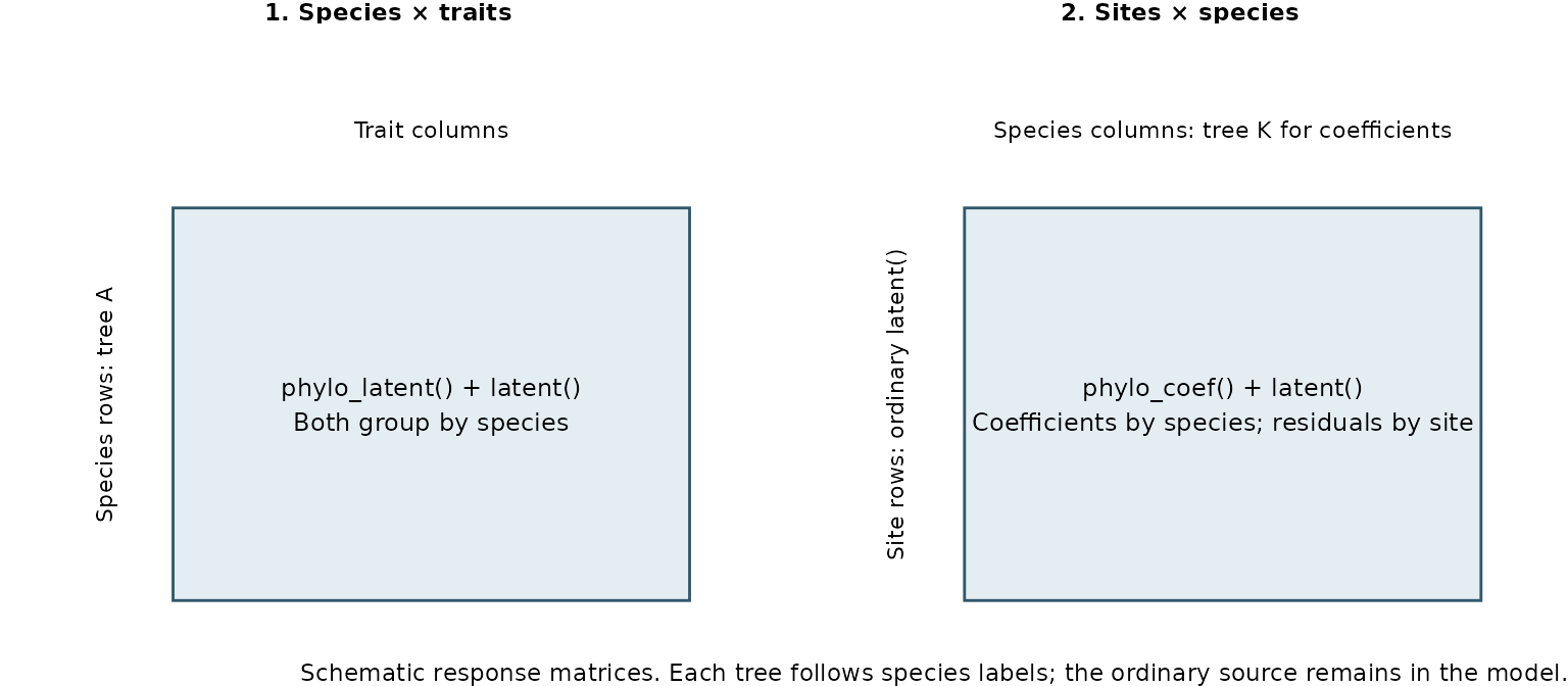
Example 1: six traits, one measurement per species
We simulate 80 species and six synthetic traits on standardized scales: leaf area, specific leaf area, leaf dry matter content, stem height, seed mass, and root depth. Each species has exactly one multivariate observation: there are no populations and no within-species variance. These are simulated scale units, not empirical measurements subsequently centred and divided by their sample SD.
Both sources are among species. The fixed effects in are trait means and trait-specific effects of standardized species elevation. is the unit-diagonal tree covariance; makes different species independent in the ordinary source. is a diagonal matrix of positive trait-specific variances. The vectorization above stacks all traits for each species together. Two latent dimensions alone do not establish separation of the sources. These equations describe the simulated components. The fitted Gaussian covariance also includes a fixed stabilizer, defined below; the simulation itself has no additional observation-error draw.
fixture <- make_tree_axis_fixture("target")
traits_morph <- fixture$morphology$traits
tree_morph <- fixture$morphology$tree
morphology <- fixture$morphology$long
morphology_wide <- fixture$morphology$wide
truth_morphology <- fixture$morphology$truth
A <- fixture$morphology$K
I <- diag(nrow(A))
source_columns <- cbind(A[lower.tri(A, diag = TRUE)], I[lower.tri(I, diag = TRUE)])
source_columns <- sweep(source_columns, 2, sqrt(colSums(source_columns^2)), "/")
c(source_rank = qr(source_columns)$rank,
  normalized_condition = kappa(source_columns, exact = TRUE))
#>          source_rank normalized_condition
#>             2.000000             1.277739
This check distinguishes the two covariance patterns algebraically. It does not guarantee accurate variance estimates from 80 species.
set.seed(202608501L)
fit_morphology <- gllvmTMB(
 value ~ 0+trait+trait:elevation+
   phylo_latent(0+trait|species,tree=tree_morph,d=2,unique=TRUE)+
   latent(0+trait|species,d=2,unique=TRUE),
 data=morphology,trait="trait",unit="species",cluster="species",
 family=gaussian(),silent=TRUE,control=fit_control
)
#> ℹ Auto-suppressing `sigma_eps`: `indep(0 + trait | species)` is at the per-row
#>   level, so it already absorbs the observation residual.
#> • Fixed at 0.00112 (~1/1000 of sd(y)) to keep the Gaussian density
#>   well-defined; the row-level residual variance is fully captured by the
#>   per-row diagonal term.
The matching wide-data call uses the same public entry point.
set.seed(202608501L)
fit_morphology_wide <- gllvmTMB(
 traits(all_of(traits_morph)) ~ 1+elevation+
   phylo_latent(1|species,tree=tree_morph,d=2,unique=TRUE)+
   latent(1|species,d=2,unique=TRUE),
 data=morphology_wide,unit="species",cluster="species",family=gaussian(),silent=TRUE,control=fit_control
)
Sphy <- extract_Sigma(fit_morphology,level="phy",part="total",link_residual="none")$Sigma
Snon <- extract_Sigma(fit_morphology,level="unit",part="total",link_residual="none")$Sigma
Sps <- extract_Sigma(fit_morphology,level="phy",part="shared",link_residual="none")$Sigma
Sns <- extract_Sigma(fit_morphology,level="unit",part="shared",link_residual="none")$Sigma
pp <- extract_Sigma(fit_morphology,level="phy",part="unique",link_residual="none")$s
pn <- extract_Sigma(fit_morphology,level="unit",part="unique",link_residual="none")$s
parts <- data.frame(trait=rep(traits_morph,4),
 component=rep(c("phylo shared","phylo diagonal","ordinary shared","ordinary diagonal"),each=6),
 variance=c(diag(Sps),pp,diag(Sns),pn))
p1 <- corplot(Sphy,"Phylogenetic trait correlation")
p2 <- corplot(Snon,"Ordinary trait correlation")
parts$trait <- factor(parts$trait, levels = traits_morph)
p3 <- ggplot(parts,aes(trait,variance,fill=component))+geom_col()+
  scale_fill_manual(values = c("phylo shared" = "#156b42", "phylo diagonal" = "#a6dba0",
                              "ordinary shared" = "#70569b", "ordinary diagonal" = "#c5afd9"))+
  labs(title="Fitted four-part variance decomposition",x=NULL,y="Variance",
       caption="Source components only; fixed observation stabilizer excluded.")+
  theme_minimal(base_size=10)+theme(axis.text.x=element_text(angle=45,hjust=1))
grid::grid.newpage(); grid::pushViewport(grid::viewport(layout=grid::grid.layout(2,2)))
print(p1,vp=grid::viewport(layout.pos.row=1,layout.pos.col=1))
print(p2,vp=grid::viewport(layout.pos.row=1,layout.pos.col=2))
print(p3,vp=grid::viewport(layout.pos.row=2,layout.pos.col=1:2))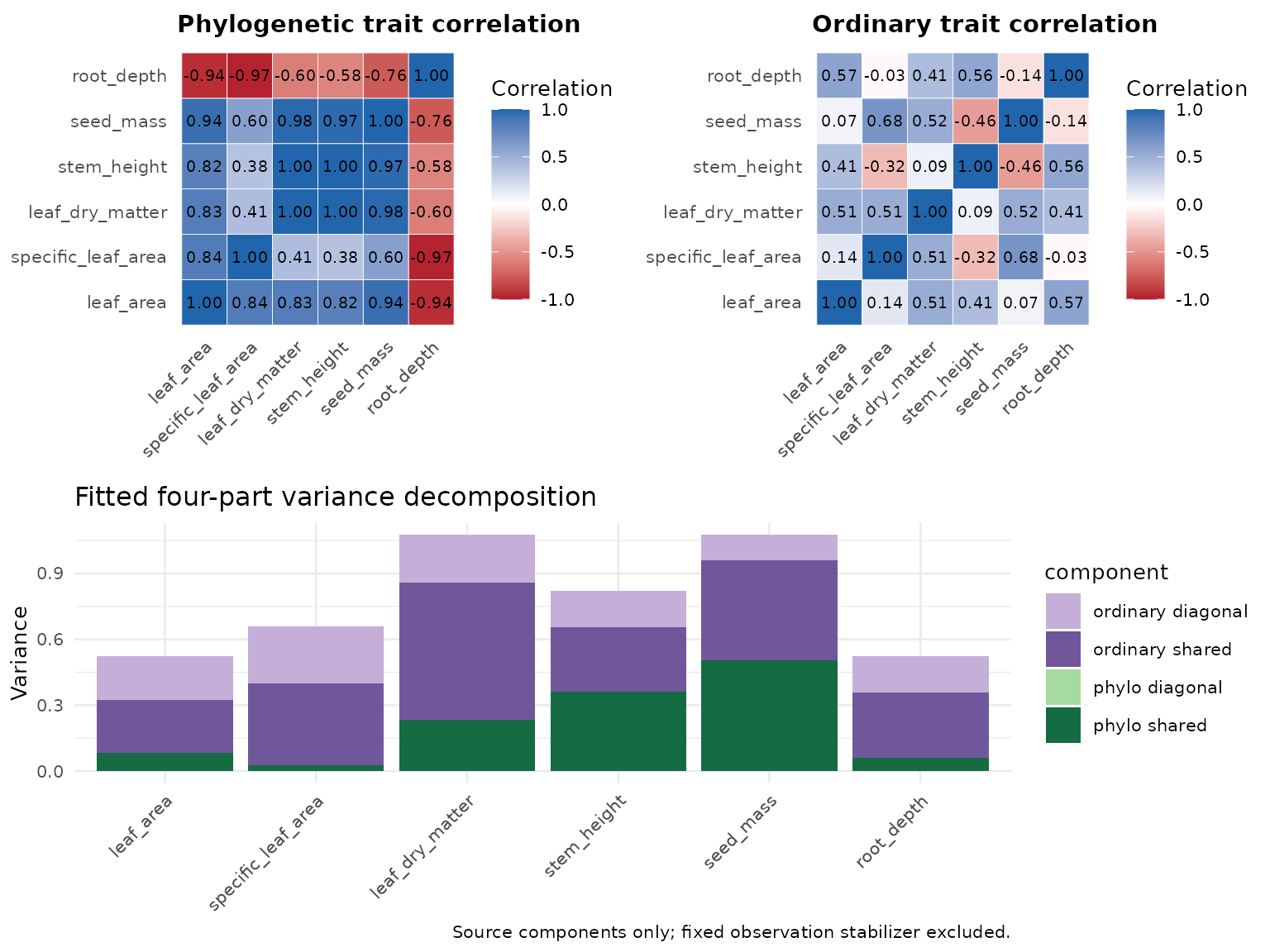
truth_estimate <- data.frame(
  trait = traits_morph,
  phylo_total_truth = diag(truth_morphology$Sigma_phy_total),
  phylo_total_fitted = diag(Sphy),
  ordinary_total_truth = diag(truth_morphology$Sigma_non_total),
  ordinary_total_fitted = diag(Snon),
  phylo_communality_truth = diag(truth_morphology$Sigma_phy_shared) / diag(truth_morphology$Sigma_phy_total),
  phylo_communality_fitted = extract_communality(fit_morphology, level = "phy", link_residual = "none"),
  ordinary_communality_truth = diag(truth_morphology$Sigma_non_shared) / diag(truth_morphology$Sigma_non_total),
  ordinary_communality_fitted = extract_communality(fit_morphology, level = "unit", link_residual = "none")
)
table_names <- c("Trait", "Phylo truth", "Phylo fitted", "Ordinary truth", "Ordinary fitted")
knitr::kable(truth_estimate[, 1:5], digits = 3, row.names = FALSE,
  col.names = table_names,
caption = "Total variance within each source. Fixed observation stabilizer excluded; one realization, not recovery evidence.")| Trait | Phylo truth | Phylo fitted | Ordinary truth | Ordinary fitted |
|---|---|---|---|---|
| leaf_area | 0.594 | 0.081 | 0.440 | 0.441 |
| specific_leaf_area | 0.506 | 0.028 | 0.567 | 0.632 |
| leaf_dry_matter | 0.609 | 0.235 | 0.645 | 0.842 |
| stem_height | 0.690 | 0.363 | 0.503 | 0.458 |
| seed_mass | 0.640 | 0.504 | 0.438 | 0.573 |
| root_depth | 0.461 | 0.059 | 0.561 | 0.464 |
knitr::kable(truth_estimate[, c(1, 6:9)], digits = 3, row.names = FALSE,
  col.names = table_names,
caption = "Communality: the shared fraction of variance within each source.")| Trait | Phylo truth | Phylo fitted | Ordinary truth | Ordinary fitted |
|---|---|---|---|---|
| leaf_area | 0.664 | 1 | 0.591 | 0.550 |
| specific_leaf_area | 0.684 | 1 | 0.559 | 0.589 |
| leaf_dry_matter | 0.606 | 1 | 0.737 | 0.742 |
| stem_height | 0.739 | 1 | 0.582 | 0.639 |
| seed_mass | 0.656 | 1 | 0.658 | 0.797 |
| root_depth | 0.696 | 1 | 0.590 | 0.643 |
The table describes one synthetic realization; it is not recovery evidence. Communality is the shared fraction of variance within one source, not that source’s share of total variance. The four-part bars show the latter components on the original variance scale. The phylogenetic diagonal estimates approach zero in this realization even though their planted values are positive; the stable fit does not establish recovery of that decomposition.
The ordinary component is between-species variation not structured by this tree. It is not automatically plot-level variation, convergence, microevolution, or measurement error. A near-zero fitted diagonal for a pre-specified source is reported, not used to alter the frozen model.
Example 2: species coefficients and residual association at sites
We simulate 150 sites and 50 species. C3 and C4 fixed pathway intercepts are .85 and .45; their latitude slopes are -.30 and .55. Species have intercept and slope deviations around those expectations. Both coefficient models retain a two-dimensional ordinary site residual component. Here denotes standardized latitude, is species ’s pathway, and contains its coefficient deviations. The response is a synthetic continuous community measurement, not a count. The contrasting pathway slopes are design assumptions, not a general claim about C3 and C4 distributions.
For the phylogenetic coefficient model,
We plant
and estimate it with rho = NULL. The tree is scaled exactly
as in Example 1, so
has unit diagonal. The coefficient standard deviations are 0.18 and
0.55, with correlation -0.25. The IID comparator uses
in place of
,
while retaining the same site covariance model. The coefficient mixture
does not describe residual co-occurrence at sites. As in Example 1, the
fitted likelihood adds the fixed observation stabilizer to the simulated
site covariance shown above.
community <- fixture$community$long
community_wide <- fixture$community$wide
column_data <- fixture$community$column_data
tree_columns <- fixture$community$tree
species_comm <- fixture$community$species
truth_community <- fixture$community$truth
set.seed(202608501L)
fit_columns <- gllvmTMB(
 value ~ 0+pathway+latitude:pathway+column_coef(1+latitude|trait)+
   latent(0+trait|site_id,d=2,unique=TRUE),
 data=community,trait="trait",unit="site_id",family=gaussian(),silent=TRUE,control=fit_control
)
#> ℹ Auto-suppressing `sigma_eps`: `indep(0 + trait | site_id)` is at the per-row
#>   level, so it already absorbs the observation residual.
#> • Fixed at 0.000846 (~1/1000 of sd(y)) to keep the Gaussian density
#>   well-defined; the row-level residual variance is fully captured by the
#>   per-row diagonal term.
set.seed(202608501L)
fit_phylo_coef <- gllvmTMB(
 value ~ 0+pathway+latitude:pathway+
   phylo_coef(1+latitude|trait,tree=tree_columns,rho=NULL)+
   latent(0+trait|site_id,d=2,unique=TRUE),
 data=community,trait="trait",unit="site_id",family=gaussian(),silent=TRUE,control=fit_control
)
#> ℹ Auto-suppressing `sigma_eps`: `indep(0 + trait | site_id)` is at the per-row
#>   level, so it already absorbs the observation residual.
#> • Fixed at 0.000846 (~1/1000 of sd(y)) to keep the Gaussian density
#>   well-defined; the row-level residual variance is fully captured by the
#>   per-row diagonal term.
set.seed(202608501L)
fit_columns_wide <- gllvmTMB(
 traits(all_of(species_comm)) ~ 0+pathway+latitude:pathway+
   column_coef(1+latitude|trait)+latent(1|site_id,d=2,unique=TRUE),
 data=community_wide,column_data=column_data,unit="site_id",family=gaussian(),control=fit_control
)
set.seed(202608501L)
fit_phylo_coef_wide <- gllvmTMB(
 traits(all_of(species_comm)) ~ 0+pathway+latitude:pathway+
   phylo_coef(1+latitude|trait,tree=tree_columns,rho=NULL)+latent(1|site_id,d=2,unique=TRUE),
 data=community_wide,column_data=column_data,unit="site_id",family=gaussian(),control=fit_control
)
The code below uses planted species curves to illustrate the simulated coefficient deviations. The current public API provides fitted coefficient covariance, not individual species coefficient modes; the curves must not be read as estimates of those modes.
fixed <- coef(fit_columns)
curve <- expand.grid(latitude=seq(-2,2,length.out=100), pathway=factor(c("C3","C4"),levels=c("C3","C4")))
X_curve <- model.matrix(~0+pathway+latitude:pathway, data=curve)
curve$mean <- drop(X_curve %*% fixed[colnames(X_curve)])
planted <- expand.grid(latitude = seq(-2, 2, length.out = 100),
                       trait = species_comm, stringsAsFactors = FALSE)
planted$pathway <- column_data$pathway[match(planted$trait, column_data$trait)]
b <- truth_community$coefficient_draw[planted$trait, , drop = FALSE]
planted$mean <- truth_community$pathway_intercept[as.character(planted$pathway)] +
  b[, "(Intercept)"] + planted$latitude *
  (truth_community$pathway_slope[as.character(planted$pathway)] + b[, "latitude"])
p1 <- ggplot() +
  geom_line(data = planted, aes(latitude, mean, group = trait, colour = pathway),
            alpha = 0.18, linewidth = 0.3) +
  geom_line(data = curve, aes(latitude, mean, colour = pathway),
            linewidth = 1.1, linetype = "dashed") +
  scale_colour_manual(values = c(C3 = "#0072b2", C4 = "#d55e00")) +
  labs(title = "Species curves and\npathway expectations",
       x = "Standardized latitude", y = "Synthetic Gaussian mean", colour = "Pathway") +
  theme_minimal(base_size = 10) +
  theme(plot.title = element_text(size = 11, face = "bold"),
        legend.position = "bottom", panel.grid.minor = element_blank())
coefphy <- extract_Sigma(fit_phylo_coef,level="column_coef")
p2 <- corplot(coefphy$Sigma,"Intercept–latitude\ncoefficient correlation")
grid::grid.newpage(); grid::pushViewport(grid::viewport(layout=grid::grid.layout(1,2)))
print(p1,vp=grid::viewport(layout.pos.row=1,layout.pos.col=1))
print(p2,vp=grid::viewport(layout.pos.row=1,layout.pos.col=2))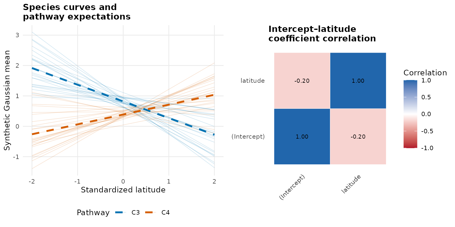
Thin lines are planted species curves; dashed lines are fitted IID pathway means. Species curves are not fitted random effects. The right panel compares intercept and latitude-slope deviations, not species pairs.
The fitted tree-mixture parameter is 2.38e-07, compared with the planted value 0.60. It describes dependence across species. The two-by-two matrix instead describes the correlation between species’ intercept and latitude-slope deviations. These are different questions. A fitted mixture near zero supplies little evidence for tree-structured coefficient variation in this realization, even though it was planted; numerical convergence alone does not demonstrate recovery.
Ssite <- extract_Sigma(fit_columns,level="unit",part="total",link_residual="none")$Sigma
p3 <- corplot(Ssite,"Site residual correlation\n(all 50 species)")
ord <- extract_ordination(fit_columns,level="unit")
scores <- as.data.frame(ord$scores); names(scores)[1:2] <- c("LV1","LV2")
p4 <- ggplot(scores,aes(LV1,LV2))+geom_point(alpha=.65)+coord_equal()+
 labs(title="Ordinary site ordination")+
 theme_minimal(base_size=10)+
 theme(plot.title=element_text(size=11,face="bold"),panel.grid.minor=element_blank())
grid::grid.newpage(); grid::pushViewport(grid::viewport(layout=grid::grid.layout(1,2)))
print(p3,vp=grid::viewport(layout.pos.row=1,layout.pos.col=1))
print(p4,vp=grid::viewport(layout.pos.row=1,layout.pos.col=2))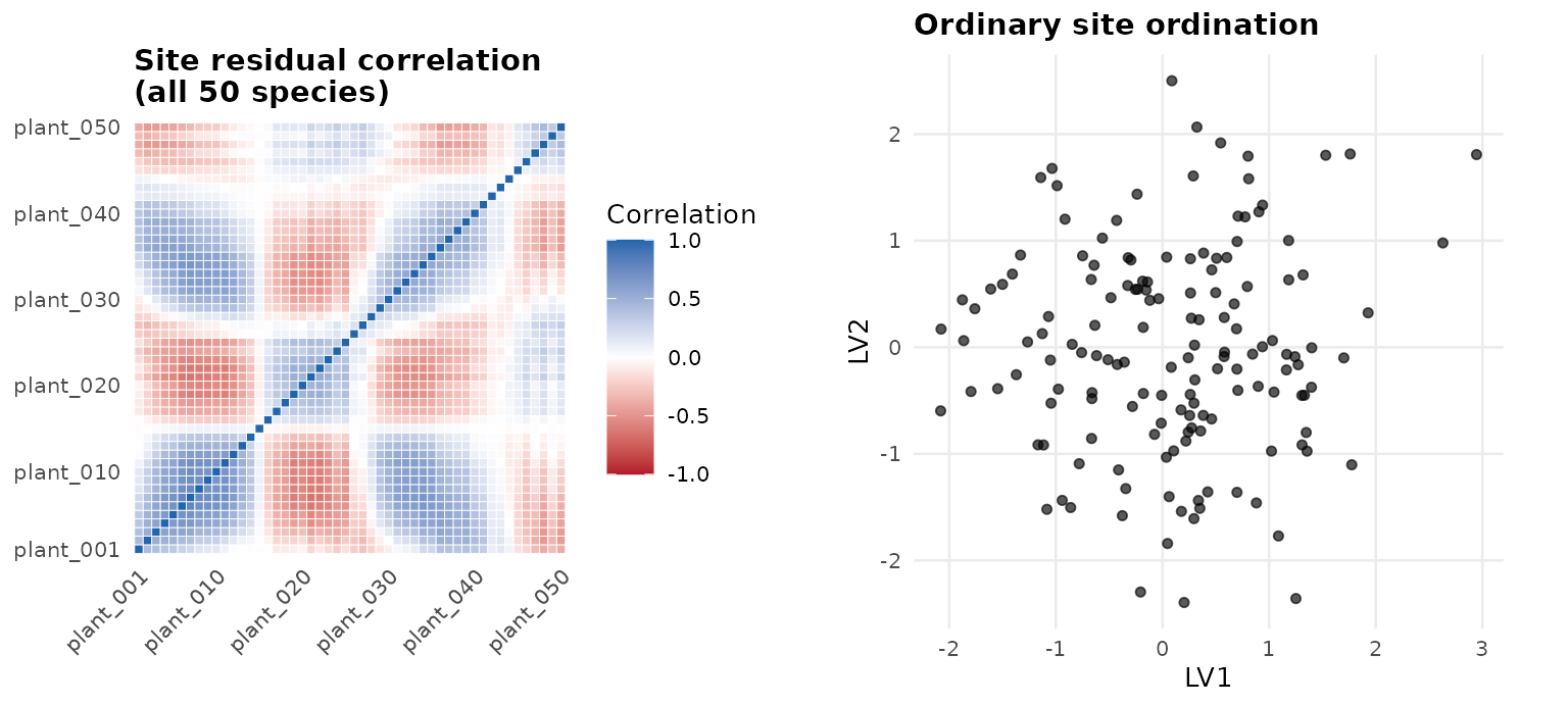
The residual matrix describes association among species responses at a site, not correlation between sites. All 50 species are shown in their fixed fixture order; only selected axis labels are printed for readability.
Residual association can arise from unmeasured environment, sampling, or shared responses. It is not proof of direct species interactions. Ordination axes can rotate or change sign and are interpreted within a fit only.
Gaussian diagonal components and scope
unique = TRUE adds a trait-specific diagonal companion
to each latent source. The phylogenetic companion still follows the
tree; it is not an independent nonphylogenetic source. The ordinary
companion groups by species in Example 1 and by site in Example 2. With
one value per group and response, it also absorbs independent cell-level
Gaussian variation. Estimating a second free observation variance would
duplicate that diagonal contribution.
The package therefore fixes the separate Gaussian residual standard
deviation to max(1e-3 * sd(y), 1e-6) for these fits, as
verified during validation. This small numerical stabilizer is not an
estimated biological component or separately identified measurement
error. control = gllvmTMBcontrol(se = FALSE) omits
standard-error calculations; it does not itself set that residual
scale.
All three models passed a bounded check using three deterministic starts, with matching long- and wide-format results. This checks numerical stability in this realization; neither example makes a recovery, interval, or causal interaction claim.