When one data source knows where it is and the other does not

The situation

You have two kinds of data on the same species. One is a large, messy pile of opportunistic records — eBird checklists, GBIF (Global Biodiversity Information Facility) occurrences — with no survey design behind it. The other is a structured monitoring programme: fewer sites, but a protocol. An integrated species distribution model (iSDM) fits both at once, on the reasoning that the structured arm can discipline the biased one (each data source inside an integrated model is called an arm – the word appears throughout these articles).

The two arms usually differ in one respect that nobody puts in the model. The opportunistic arm knows where it is; the survey arm often does not.

This is not sloppiness — it is policy. Monitoring programmes routinely publish coordinates degraded on purpose, to protect site access agreements and to avoid disclosing the locations of species at risk. ABMI, the Alberta Biodiversity Monitoring Institute, publishes public survey locations blurred to roughly 5.5 km, and coarser still for sensitive species; precise coordinates require a separate data agreement. An eBird checklist in the same landscape carries a GPS fix. The two arms are then fused as though both located their observations equally well, and one of them did not.

Throughout this article that deliberate blurring is called fuzz, and it is measured not in kilometres but relative to the habitat layer — for reasons that become the whole point below.

This is a documented problem, not a hypothetical one. Work on iNaturalist’s obscured-geoprivacy setting reports that obscured locations change the environmental values attached to a record — elevation, habitat type, extracted covariates — and change the resulting estimated distributions (Koo et al. 2025). Gábor et al. (2022) likewise find that SDM performance degrades as positional error in occurrence records grows.

Why the spatial random field does not rescue you

The reason fuzzed coordinates still feel harmless in an integrated model is a sensible-sounding intuition: there is a spatial random field in the model, positional error is spatial noise, so the field will absorb it. That intuition is about the response. The damage is to the covariate.

Environmental predictors in an SDM are almost never measured at the site. They are extracted from a raster at the recorded coordinate. If the recorded coordinate is wrong by 5.5 km you read temperature, elevation or canopy cover from the wrong place, and then regress the species’ response — which happened at the true location — on a habitat value from a different one.

The consequence is well known and has a name. When a predictor is measured with error, the estimated slope on that predictor is dragged toward zero: the habitat effect looks weaker than it really is. Statisticians call the situation errors-in-variables and the symptom attenuation; both terms are used below, and both mean what the previous sentence says. Nothing about the mechanism is new here. What this article measures is what the mechanism does inside a two-arm integrated fit, and what decides whether you should care.

That last part is not decided by the fuzz in kilometres. It is decided by the fuzz relative to how far you have to move before the habitat layer stops looking like itself. Five and a half kilometres is nearly nothing across a smooth continental temperature gradient, and severe across a patchy canopy-cover layer. So that ratio comes first, before any simulation.

The number that decides it

The number is your survey arm’s positional uncertainty divided by the correlation length of the habitat layer you care about — the distance over which values in that layer stay similar to each other.

Getting that number wrong by a factor of three is enough to flip the recommendation, and a factor of three is exactly what sits between the two quantities that software calls “range”. So it is worth being exact about which one is meant.

For a covariate whose spatial correlation behaves like exp(-d / phi), phi is the distance at which the covariate’s correlation with itself falls to 1/e ≈ 0.368. That is what “correlation length” means here, and it is computable directly from a raster. Software that fits a variogram – the standard geostatistical plot of how similarity between raster values decays with distance – commonly reports instead the practical range, conventionally about 3 * phi, the distance at which correlation falls to 0.05. Dividing a reported practical range by 3 before comparing it to your positional fuzz is the single most important arithmetic step in applying this article to your own data.

The recipe

The function below measures phi from a set of cells. It works by building a correlogram — the average correlation between pairs of cells, binned by how far apart they are — and then reading off the distance at which that curve crosses 1/e.

## phi = the distance at which the covariate's own spatial correlation falls
## to 1/e. NOTE n_sub: this builds a dense n x n distance matrix, so it takes
## a SUBSAMPLE of cells, never a whole raster.
cor_length <- function(x, y, z, n_bin = 30, n_sub = 2000, seed = 1) {
  if (length(x) > n_sub) {
    ## Subsample reproducibly WITHOUT clobbering the caller's RNG stream: a
    ## bare set.seed() here would change every random draw you make
    ## afterwards, invisibly.
    old <- if (exists(".Random.seed", .GlobalEnv))
      get(".Random.seed", .GlobalEnv) else NULL
    set.seed(seed)
    i <- sample.int(length(x), n_sub)
    if (is.null(old)) rm(".Random.seed", envir = .GlobalEnv) else
      assign(".Random.seed", old, envir = .GlobalEnv)
    x <- x[i]; y <- y[i]; z <- z[i]
  }
  d   <- as.matrix(dist(cbind(x, y)))
  cp  <- outer(z - mean(z), z - mean(z)) / var(z)
  ut  <- upper.tri(d)
  brk <- seq(0, quantile(d[ut], 0.5), length.out = n_bin + 1)
  rho <- tapply(cp[ut], cut(d[ut], brk, include.lowest = TRUE), mean)
  h   <- (brk[-1] + brk[-length(brk)]) / 2
  ok  <- !is.na(rho); rho <- rho[ok]; h <- h[ok]

  ## Walk outward to the FIRST crossing of 1/e and interpolate there.
  ## approx(rho, h, xout = 1/e) would sort on the correlations, and a measured
  ## correlogram does not fall monotonically -- sorting silently re-pairs
  ## distances with correlations they did not come from.
  below <- which(rho < exp(-1))
  if (!length(below))
    stop("cor_length(): the correlogram never falls to 1/e within half the ",
         "maximum inter-point distance. phi is too long to measure on this ",
         "extent -- your covariate is smoother than your map is wide. ",
         "Use a larger region, and do not substitute the largest distance ",
         "you can see.", call. = FALSE)
  k <- below[1]
  if (k == 1L)
    stop("cor_length(): correlation is already below 1/e in the first ",
         "distance bin, so phi is shorter than the spacing between the cells ",
         "supplied. Supply finer cells; do NOT read the returned bin ",
         "midpoint as phi.", call. = FALSE)
  h[k - 1] + (rho[k - 1] - exp(-1)) / (rho[k - 1] - rho[k]) * (h[k] - h[k - 1])
}

Do not hand it a whole raster, and do not coarsen one to make it fit. Both halves matter. The distance matrix grows with the square of the number of cells, and that arithmetic is unforgiving: n cells cost 8 * n^2 bytes per matrix, so 22,500 cells is 3.8 GB and a 1 km Alberta raster (~10⁶ cells) would need 7 TB. The n_sub argument takes a random subsample instead, and a subsample is enough. terra::aggregate() is the wrong fix, and it fails in the dangerous direction: coarsening inflates the estimated phi, which shrinks your fuzz-to-phi ratio and makes your situation look safer than it is. Subsample cells; do not average them. (Coarsening is also not a remedy for the underlying problem — see What to do.)

Here it is working on a surface whose phi is known by construction, and then refusing to answer on one it cannot measure:

sim_surface <- function(n_side, phi, seed) {
  set.seed(seed)
  gx <- seq(0, 1, length.out = n_side)
  g  <- expand.grid(lon = gx, lat = gx)
  S  <- exp(-as.matrix(dist(g)) / phi)
  g$z <- as.numeric(scale(as.numeric(
    t(chol(S + diag(1e-6, nrow(S)))) %*% rnorm(nrow(g)))))
  g
}

g <- sim_surface(41, phi = 0.05, seed = 1)     # cell spacing 1/40 = 0.025
cor_length(g$lon, g$lat, g$z)                  # true phi = 0.05
#> (0.035,0.0526] 
#>     0.05249077

g_coarse <- sim_surface(21, phi = 0.02, seed = 1)   # cell spacing 0.05 > phi
try(cor_length(g_coarse$lon, g_coarse$lat, g_coarse$z))
#> Error : cor_length(): correlation is already below 1/e in the first distance bin, so phi is shorter than the spacing between the cells supplied. Supply finer cells; do NOT read the returned bin midpoint as phi.

The second call is the important one. The cells are further apart than the correlation length, so the correlogram is already below 1/e in its first bin and there is nothing to interpolate. The function stops and says which of the two ways it failed, rather than returning a number you would have no reason to distrust.

Where the recipe can be trusted

Two things can go wrong, and they are different: phi can be long relative to your map, or short relative to your cells. The grid below crosses those two so they can be told apart — twelve simulated surfaces per cell, each with a phi that is known exactly.

phi / map width	phi / cell spacing	refused (of 12)	mean phi_hat / phi	sd over surfaces	above truth
0.02	0.4	12	NA	NA	0 / 0
0.02	0.8	12	NA	NA	0 / 0
0.02	1.2	0	0.711	0.108	0 / 12
0.05	1.0	9	1.043	0.132	2 / 3
0.05	2.0	0	1.024	0.141	7 / 12
0.05	3.0	0	0.996	0.110	4 / 12
0.10	2.0	0	0.894	0.198	4 / 12
0.10	4.0	0	0.950	0.177	3 / 12
0.10	6.0	0	0.895	0.119	4 / 12
0.25	5.0	0	0.705	0.213	1 / 12
0.25	10.0	0	0.757	0.171	1 / 12
0.25	15.0	0	0.685	0.196	1 / 12
0.40	8.0	0	0.526	0.140	0 / 12
0.40	16.0	0	0.555	0.135	0 / 12
0.40	24.0	0	0.516	0.134	0 / 12

mean phi_hat / phi is the recipe’s answer divided by the truth, so 1.00 is perfect and anything below 1 means the recipe read short. Read down the table and then across it.

Down — the bias belongs to the map’s width. As phi grows relative to the map, the recipe reads low: about 0.72 × truth at phi a quarter of the map’s width, 0.53 × at four tenths. Read across at a fixed phi / map width and the three lattice resolutions give essentially the same answer. That is what makes it a map-size effect and not a resolution one: a correlation longer than your map cannot be seen on your map.

Across — the resolution decides whether you get an answer at all. Once phi falls to about the spacing between your cells, the recipe refuses on every surface or nearly every one. The row that answers at phi / cell spacing = 1.2 should be read as a warning rather than a success: it returns a number, and the number is 29% low.

The error is not reliably downward on a single raster. The column means above are means over twelve surfaces, and it is tempting to read “reads low” as a guarantee for your one raster. It is not. Even in the region where this recipe is recommended — phi at or under a tenth of the map and at least twice the cell spacing — the surface-to-surface standard deviation of phi_hat / phi is 0.11–0.20, and 22 of 60 individual surfaces (37%) come out above truth. Run the recipe on several covariate layers or several subsamples, and do not read the third significant figure.

So, operationally. Trust it when phi sits comfortably below a tenth of your study region’s width and comfortably above your cell spacing. Outside that window it either refuses or reads low. Reading low inflates your computed fuzz / phi ratio, which for this article’s decision errs toward looking more carefully — but that is not a licence to treat the number as exact.

What actually happens

The design

Two species share a landscape with a single smooth habitat surface. Counts are generated from the habitat value at each site’s true location, with a shared slope $\beta = 0.9$ — that is the number every estimate below is trying to recover. The presence-only arm records its coordinates exactly. The survey arm’s recorded coordinates are displaced by noise whose standard deviation is fuzz × the correlation length, so fuzz = 0.5 means “displaced by about half the distance over which the habitat layer stays similar to itself”.

The covariate handed to the model is then read at each arm’s recorded location, which is what an analyst would do. Three analyses of the identical world are compared — precise (the presence-only arm alone), fuzzed (the survey arm alone) and integrated (both together, the thing an iSDM does) — at three fuzz levels and three arm-size designs, 15 replicate landscapes each.

Three features of the design worth knowing before reading the numbers:

• No spatial field is fitted. Fixed effects only. This isolates the covariate channel cleanly, and it means the article does not measure how much of the damage a fitted field would absorb — the intuition named at the top is set aside here, not tested.
• The precise arm is generated before fuzz is used, so its estimate is identical to the last digit across the three fuzz levels (0.91191458 at all three in the 100/400 design). Its flat line in the figure is therefore built in, not a result. It buys perfect pairing between the three analyses, which is the point.
• The three designs share their 15 landscapes (the same replicate seeds). They are three designs on one set of landscapes, not 45 independent trials.

The measurement

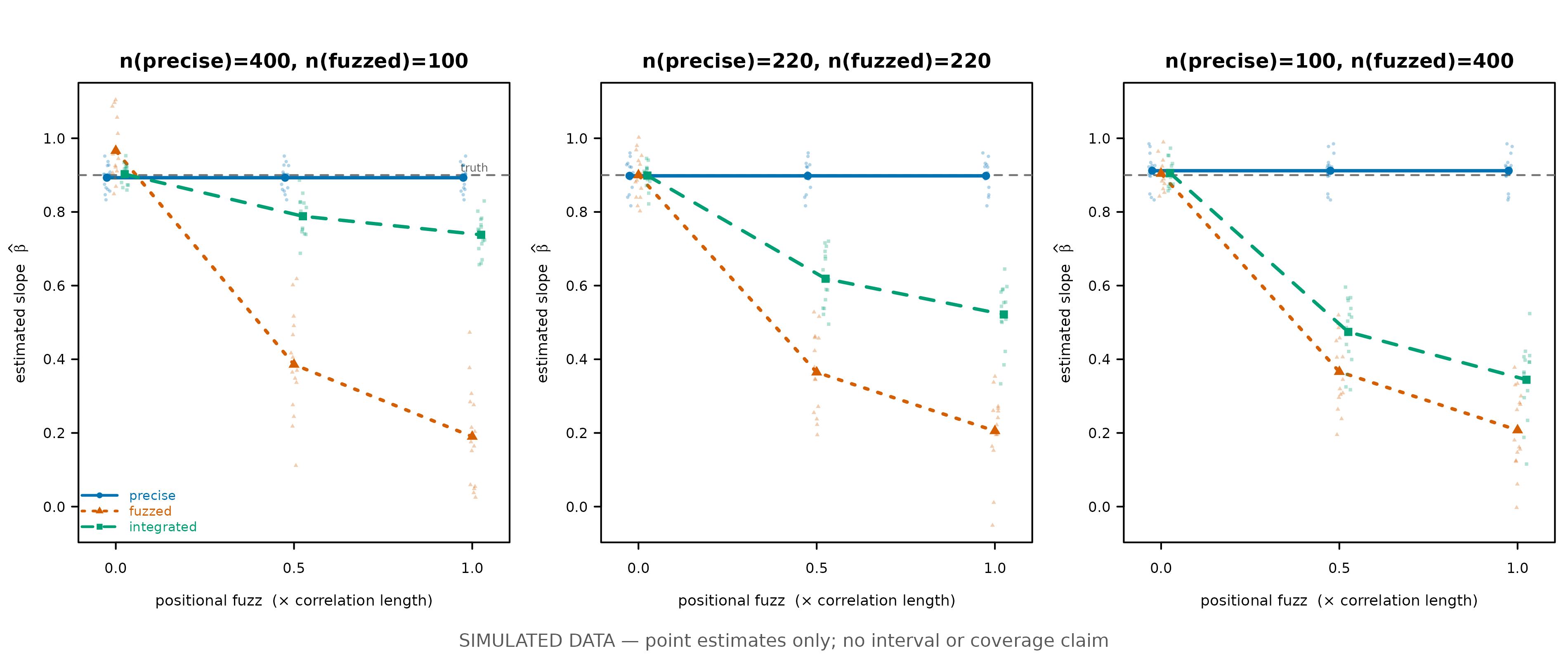
The attenuation penalty across three arm-size designs, each n(precise) / n(fuzzed), ordered left to right by the FUZZED arm’s share of the data: 400/100 (fuzzed arm one fifth), 220/220 (equal), 100/400 (fuzzed arm four fifths, a stress test). Pale symbols are the 105 distinct fits behind each design - 15 precise (generated before fuzz is applied, so the same 15 are drawn at each fuzz level), 45 fuzzed and 45 integrated. Solid symbols and lines are the design’s arm means. The dashed grey line, labelled in the first panel, marks the true slope 0.9. In every design the precise arm sits at truth and the fuzzed arm collapses toward zero; the integrated fit falls between them at a depth set by how much of the pooled data the fuzzed arm supplies.

The same numbers as a table, since a figure is read and a table is checked. Mean estimated slope (true value 0.9), with the arm-size-weighted average of the two single-arm means alongside the integrated fit:

n(precise)	n(fuzzed)	fuzz	precise	fuzzed	integrated	n-weighted avg
400	100	0.0	0.893	0.966	0.903	0.908
400	100	0.5	0.893	0.386	0.788	0.792
400	100	1.0	0.893	0.190	0.738	0.752
220	220	0.0	0.898	0.900	0.899	0.899
220	220	0.5	0.898	0.365	0.619	0.631
220	220	1.0	0.898	0.205	0.522	0.552
100	400	0.0	0.912	0.904	0.906	0.906
100	400	0.5	0.912	0.366	0.474	0.475
100	400	1.0	0.912	0.208	0.344	0.348

The fuzzed arm is gutted. Displaced by half the correlation length, it has already lost 57–59% of the true slope; displaced by a full correlation length, 77–79%. Across all six non-zero cells the loss is 57–79%. That is the finding. Everything else follows from it.

Pooling behaves exactly as pooling should. The integrated estimate lands between the two single-arm estimates, which is what averaging does — the last column of the table is the arm-size-weighted average of the two single-arm means, and it tracks the integrated fit to within 0.018–0.041 within each replicate, in every design including the unbalanced ones. There is nothing pathological in the fitting.

The problem is what is being averaged in. The fuzzed arm arrives carrying 57–79% attenuation, and the pooled estimate inherits it in proportion to that arm’s share of the data. Hold fuzz at 0.5 and grow the fuzzed arm’s share — 100 rows against 400, then 220 against 220, then 400 against 100 — and the gap integrated − precise deepens in step: -0.105 → -0.279 → -0.438, with non-overlapping confidence intervals ([-0.126, -0.083], [-0.313, -0.246], [-0.486, -0.390]).

The general mechanism is already documented. Fletcher et al. (2019) show that in integrated SDMs without explicit weighting, estimates are largely driven by the abundant presence-only data, increasingly so as that arm grows — the integrated model’s parameters shrink toward the presence-only model’s. That is swamping. What this article adds is narrower: positional error is one of the defects that gets swamped in, the attenuation it causes is severe well before the fuzz reaches the covariate’s correlation length, and the ratio in the previous section is what tells you whether your case is in that regime.

The zero-fuzz control mostly works, and where it does not, the cause is identifiable. Eight of the nine arm means at fuzz = 0 sit within 0.012 of truth. The ninth is the fuzzed arm in the 400/100 design, at 0.966 — 3.02 standard errors above 0.9, p = 0.009, so it is not noise. It is the smallest arm in the grid (100 sites) at log-scale intercepts of −0.3 and 0.1, i.e. counts of order one, which is the regime where the Poisson maximum-likelihood slope is biased upward in small samples. The control still does its job — the large bias appears only when positional error does — but this one cell is a known small-sample effect rather than a fluke.

Landscape by landscape, integration loses. The precise-arm and integrated analyses saw the same landscape and the same truth, so they can be paired. Counting how often the integrated estimate is simply lower, it is lower in 15 of 15 replicates in every design at both non-zero fuzz levels. Counting how often it is further from the truth — the quantity that actually matters — it is worse in 14 of 15 in the 400/100 design at fuzz = 0.5 and in 15 of 15 everywhere else. The two counts differ in one cell out of six, and the smaller one is the one to quote.

With a biased opportunistic arm

Everything above gives the opportunistic arm a property that removes the whole reason anyone integrates: it is unbiased. Nobody fuses a structured survey with an opportunistic pile for fun. They do it because the opportunistic arm is biased by accessibility, effort and detectability, and the structured arm is what corrects that. Taken at face value, the result above could leave you concluding that your survey arm is not worth keeping — so the design is repeated with that motivation put back in.

In this second run the opportunistic arm is precise but sampling-biased: reporting intensity carries a coefficient of 1.2 on an accessibility surface drawn independently of the habitat covariate. The survey arm is unbiased but fuzzed, as before. The analyst models the bias with an access term, as a competent one would — accessibility is observable in real analyses (road density, trail networks) even though the reporting bias it induces is not.

The two surfaces are independent by construction, but each replicate draws its own pair, so the correlation actually realised in any one landscape varies: across the 15 landscapes it runs from -0.28 to 0.20 (mean -0.01, sd 0.15). The whole range is quoted because a single seed’s value would suggest the design pins it at zero, and it does not.

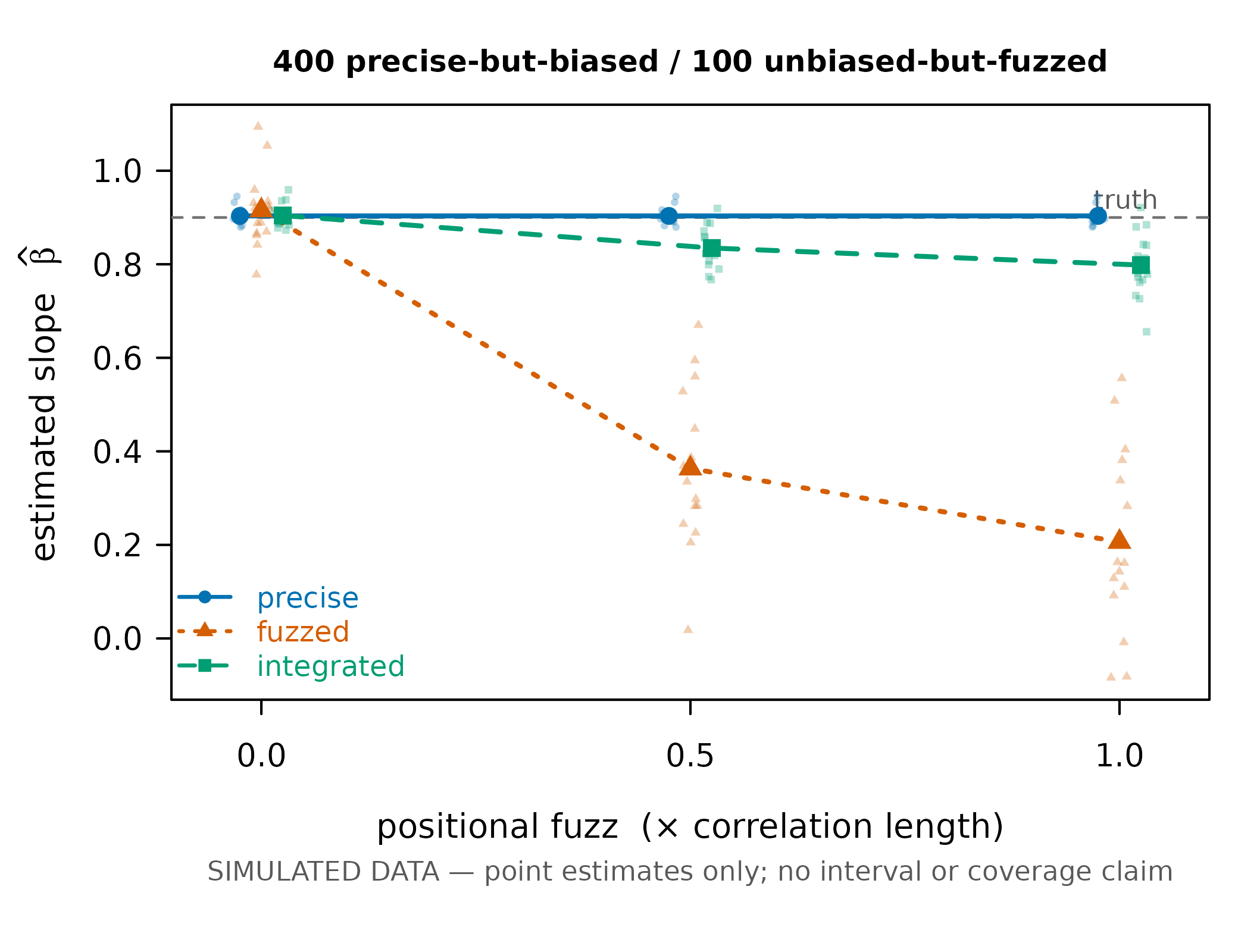
The same penalty with a precise but sampling-biased opportunistic arm (400 rows, reporting intensity biased by accessibility) against an unbiased but fuzzed survey arm (100 rows). Pale symbols are the 105 distinct fits (15 precise, generated before fuzz is applied and so drawn at each fuzz level; 45 fuzzed; 45 integrated); solid symbols and lines are means. The bias is modelled with an access term in every fit. The integrated estimate still falls below the precise-arm-alone estimate at both non-zero fuzz levels, by a smaller margin than in the unbiased design.

fuzz	precise (biased)	fuzzed (unbiased)	integrated	integrated - precise	lower (of 15)	further from truth (of 15)
0.0	0.903	0.915	0.904	0.001	10	10
0.5	0.903	0.363	0.835	-0.069	14	14
1.0	0.903	0.206	0.798	-0.105	14	15

The penalty survives the realistic design. With the motivation for integration present and correctly modelled, integrating the fuzzed arm still moves the habitat slope further from truth in 14 of 15 replicates at both non-zero fuzz levels. The gap is smaller than in the unbiased design — but do not compare the magnitudes across the two runs: this one fits an access term the other does not, so they are different models, and only the within-run contrast is valid in each.

The finding is also narrower than it may sound. The penalty falls on the habitat slope specifically. The same survey arm, once its coordinates are fuzzed, damages that slope while it repairs the reporting bias. Both are true at once, and which one wins is the next section. It matters, because the answer changes sign.

When the conclusion reverses

Read this section if you read nothing else. Everything so far has given the simulation something no real analysis has: the accessibility surface — the thing that explains where people happened to record — is measured exactly, and put in the model. Given that, the presence-only arm’s habitat slope is already unbiased, so adding a fuzzed arm can only cost you. Every number above is a cost with no benefit to weigh against it.

Real data never gives you that. You proxy “where people record” with road density, trail networks, effort — surrogates that are (a) measured imperfectly and (b) correlated with your habitat layer, because roads follow terrain and land cover. When both of those are true at once, the ranking flips: the fuzzed survey arm earns its place. Integrating it moved the habitat slope closer to truth in 11 of 12 landscapes, against 0 of 12 when the same surrogate was measured exactly. Drop the survey arm in that situation and you will probably do worse, fuzz and all.

Two things to hold on to before taking that as licence. It needs both problems together, not either one alone — an imperfect surrogate that happens to be unrelated to habitat does not flip anything. And in the regime where the flip happens, neither answer is close to the truth; “integration helped” means “less wrong”, not “right”. Both points are measured below.

What was varied

One thing changes at a time, 12 replicate landscapes each, all at fuzz = 1.0 — the worst case measured above. The five rows are:

• measured exactly — the baseline used in the previous section: the accessibility surface is unrelated to habitat and known without error.
• surrogate error only — the surrogate is measured with error (sd 0.5) but is still unrelated to habitat.
• confounding only — the surrogate is correlated with habitat (cor = 0.7) but is measured exactly.
• confounding + surrogate error — both at once. This is the row that resembles real data.
• confounded, not modelled — the surrogate is correlated with habitat and the analyst leaves it out of the model altogether.

what the analyst has	cor(access, env)	surrogate error sd	precise	precise-arm bias t	integrated	integration helped
measured exactly	0.0	0.0	0.918	1.56	0.806	3 / 12
surrogate error only	0.0	0.5	0.863	-1.24	0.787	3 / 12
confounding only	0.7	0.0	0.910	1.24	0.812	0 / 12
confounding + surrogate error	0.7	0.5	1.192	6.33	1.083	11 / 12
confounded, not modelled	0.7	0.0	1.722	10.05	1.577	12 / 12

precise-arm bias t is how many standard errors the presence-only-alone slope sits away from the true 0.9; roughly, values beyond about 2 in absolute value say that arm is biased on its own. integration helped counts the landscapes in which the integrated estimate was closer to 0.9 than the presence-only arm alone.

Reading the table

Neither problem flips it alone. An imperfect surrogate by itself, with accessibility unrelated to habitat, leaves the presence-only slope unbiased (row 2, bias t below 2 in absolute value) and integration helps in 3 of 12 — no different from the 3 of 12 baseline (Fisher p = 1.00). Correlation with habitat by itself, with the surrogate measured exactly, helps in 0 of 12. Only when the surrogate is both imperfect and correlated with habitat does the ranking reverse, to 11 of 12 (p = 9.6e-06 against correlation alone).

That is exactly what measurement error in a regressor is expected to do: error in one predictor spills into another predictor’s coefficient only through the covariance between them. It is also a more useful instruction than a general warning, because the condition is one you can check rather than assume. Compute cor(env, surrogate) on your own data. Road density is correlated with almost every environmental layer, so in practice the warning usually applies — but now you can tell.

Treat the table as one comparison, not four ranked results. Twelve landscapes per row is not many, and the proportions are correspondingly imprecise: 11/12 is [0.615, 0.998] and 3/12 is [0.055, 0.572]. With counts this small, rows 1 and 2 cannot be told apart from each other, and neither can rows 4 and 5. The one comparison the design can actually resolve is correlation-alone against correlation-plus-error.

And the bottom two rows say something else that matters: in that regime nothing recovers the truth. Precise 1.19, integrated 1.08, against a true 0.9. The ranking flips; both answers are still bad.

So the decision this article supports is narrower than the measurement driving it. Positional precision is a cost to measure, not a reason to discard a structured arm. If your bias surrogate is imperfect and correlated with your habitat layer — and for road-density-style surrogates it usually is — the structured arm is probably earning its place despite the fuzz.

What to do

gllvmTMB does not implement a fix and this article does not claim one. The general remedy is an errors-in-variables layer with a per-arm positional prior: a real modelling option, and not implemented here.

1. Compute the ratio, do not eyeball the map. Run the recipe on your own raster, divide any reported practical range by 3 first, and compare the result to your survey arm’s positional uncertainty. Fuzz well below the correlation length is benign; by half the correlation length the tables above already show 57%+ attenuation in the affected arm.
2. Check cor(env, surrogate). It decides which way the previous section points for you. Surrogate unrelated to habitat: the fuzzed arm is a net cost. Correlated with habitat and imperfectly measured: it is probably a net gain.
3. Weight the arms, or at least know what the unweighted fit is doing. The penalty tracks the fuzzed arm’s share of the pooled data, so an integrated fit that lets the larger arm dominate is making that choice implicitly. Fletcher et al. (2019) reach the same conclusion from the swamping side.
4. Fit the arms separately first. If the precise-arm-alone and integrated slopes disagree materially, that gap is evidence rather than noise. In real data it can reflect positional error, sampling bias, detection differences, or a genuine scale difference all at once, and these clean simulations cannot tell you which.
5. Ask for the precise coordinates. Most fuzzing regimes, ABMI’s included, have a data-agreement route to exact locations. For an analysis that turns on a habitat slope, that request is worth making before the analysis rather than after.

Do not reach for the obvious mitigation, because it has been tested and it does not work. The intuitive fix is to match covariate resolution to positional precision — if coordinates are fuzzed to 5.5 km, extract covariates at 5.5 km, so they are read at approximately the right place. Gábor et al. (2022) tested that directly, and the answer is in their title: positional errors in species distribution modelling are not overcome by the coarser grains of analysis. Moudrý et al. (2023) restate the same finding. Coarsening destroys fine-scale signal and does not buy back what positional error took, so it costs twice. Measure the ratio, and treat the positional error as a property of the data rather than something a resolution choice can absorb.

A related defect worth checking while you are there. Positional error corrupts the covariate at fit time. Scaling that covariate separately on the training data and on a prediction grid corrupts it at prediction time — a different error with the same flavour. That one is affine, so it preserves the map’s rank order exactly: every hotspot stays a hotspot and nothing warns you, while the predicted values themselves shift by an amount that depends on the two datasets’ means and standard deviations. The companion isdm-canada-warbler article shows the fix.

Scope and limits

• Everything here is simulated, and that is a hard boundary rather than a caveat. No real ABMI or GBIF data was fitted anywhere in this article. The 5.5 km figure is documented ABMI policy and motivates the design; it is not a measurement of bias in any real dataset.

• The displacement is clipped at the edge of the map, so the fuzz axis is slightly mislabelled. Displaced coordinates are pushed back inside the unit domain, so at fuzz = 1.0 about 36% of survey rows are clipped on at least one axis and the displacement actually realised is about 85% of nominal (19% and 93% at fuzz = 0.5). The axis labels are therefore off by roughly 10–15%, in the conservative direction — the fuzzed arm is if anything less damaged than the label implies. Real administrative fuzzing is often uniform-within-a-cell or grid-snapped, which will behave differently again.

• One covariate structure. A single smooth surface with exponential correlation. Patchier or directional covariates will attenuate differently.

• The simulated landscape sits where the recipe reads low. Its phi is 0.25 of the domain side, so a reader applying this article’s own recipe to this article’s own landscape would get about 0.18 rather than 0.25, and would read the fuzz = 1.0 cell as a ratio near 1.4 rather than 1.0. That is exactly the arithmetic the article asks you to perform, so it is stated here rather than left to be discovered.

• Fixed effects only. No spatial field is fitted in either design, which isolates the covariate channel and means the field-absorption intuition from the opening is set aside, not tested. Positional error also corrupts an estimated spatial field; that is not measured here.

• One bias mechanism. One accessibility surface, one bias coefficient. Real reporting bias may be multi-causal, non-linear, or itself measured with error.

• Fifteen replicates, and three designs on one set of landscapes. The effects reported are large relative to their confidence intervals, but the three designs are not three independent confirmations, and no number here is a precision estimate.

• No coverage claim. Point estimates only. Whether confidence intervals around these attenuated slopes retain their nominal coverage is a separate question, and it is not answered here.

References

• Fletcher, R. J. Jr., Hefley, T. J., Robertson, E. P., Zuckerberg, B., McCleery, R. A., & Dorazio, R. M. (2019). A practical guide for combining data to model species distributions. Ecology, 100(6), e02710. Establishes that unweighted integrated models are driven by the abundant presence-only arm, increasingly so as that arm grows.
• Koo, K. S., Lee, K.-H., Lee, D., & Jang, Y. (2025). Impact of obscured data on species distribution models. Conservation Biology, 39, e70050. The direct test of iNaturalist’s obscured-geoprivacy setting: obscuring changed the environmental values attached to records and the estimated distributions of three endangered species.
• Gábor, L., Jetz, W., Lu, M., et al. (2022). Positional errors in species distribution modelling are not overcome by the coarser grains of analysis. Methods in Ecology and Evolution, 13, 2289–2302. Also reports SDM performance declining as positional error grows.
• Moudrý, V., Keil, P., Gábor, L., et al. (2023). Scale mismatches between predictor and response variables in species distribution modelling: A review of practices for appropriate grain selection. Progress in Physical Geography: Earth and Environment, 47, 467–482. Restates the Gábor et al. result in a review of spatial-resolution choices in species distribution modelling.

Evidence behind the results

Every numerical statement on this page is calculated from retained replicate-level results. The evidence comprises the three arm-size designs, the sampling-biased opportunistic-arm study, the surrogate-error reversal, and the correlation-length accuracy grid described above.

The correlation-length study crosses map width with cell spacing because the two failure modes are different. Results are reported across individual surfaces rather than only as a mean, and paired comparisons use distance from the truth as well as sign. The surrogate-error-only comparison isolates the mechanism behind the reversal. Finally, this page does not recommend matching covariate resolution to positional precision: Gábor et al. (2022) tested that idea and found that coarsening does not remove positional-error bias.