Phylogenetic ordinal and nominal PGLMMs

Mizuno, Drobniak, Williams, Lagisz & Nakagawa (2025, J. Evol. Biol. 38:1699-1715, doi:10.1093/jeb/voaf116) is a tutorial on phylogenetic generalized linear mixed models (PGLMMs) for discrete traits — ordinal (threshold) and nominal (unordered) categories — implemented with MCMCglmm and brms. This article works through the paper’s two worked examples in gllvmTMB: a fast frequentist route to the same models, using the paper’s own archived data (https://github.com/Ayumi-495/PGLMM_tutorial, Zenodo 10.5281/zenodo.17038830, CC BY 4.0).

The recovery numbers below describe these two real bird datasets, fitted once. They are worked examples, not a calibration study — no interval here is certified to cover at any nominal rate (see “What this article does not claim” at the end).

Setup and data

library(gllvmTMB)
library(ggplot2)

The data layer fetches the paper’s archived CSVs and Nexus trees to a local cache (never into the package or the git history — the trees are Jetz/BirdTree-derived with no explicit licence) and validates the schema after every fetch: expected columns, the three documented Migration levels, and exact tree-tip/species matching. If a fetch fails and no cache exists, the loader returns NULL with an explanatory message instead of stale or partial data, and the examples below are skipped visibly rather than silently.

Example 1 — a phylogenetic ordinal (threshold) PGLMM

The paper’s ordinal example (their section 3) regresses a three-level migratory-behaviour trait on body mass in accipitrid raptors (Accipitridae, 136 species, one row per species, a Jetz/BirdTree phylogeny). gllvmTMB is a multivariate engine: every covariance-structure keyword (phylo_latent(), phylo_indep(), phylo_dep(), …) builds its design matrix through a trait factor, and that factor needs at least two levels — a genuinely single-trait (univariate) fit of this kind is out of gllvmTMB’s scope and belongs to glmmTMB or the paper’s own MCMCglmm/brms route (see “What this article does not claim”).

So this article lifts the example to a genuine bivariate ordinal PGLMM, pairing Migration_ordered with a second real trait from the same table, Habitat.Density (open/semi-open/dense, also three levels). The pairing has a real biological question behind it, not just a workaround: migratory raptors are disproportionately birds of open country, so a shared phylogenetic axis between migratory tendency and habitat openness is a reasonable hypothesis, testable directly from the fitted phylogenetic correlation below. Body mass (log-scale) stays in the model as a covariate on both traits, as in the paper.

d1 <- ex1$data
df_long <- rbind(
  data.frame(species = d1$species, trait = "migration",
             value = as.integer(d1$Migration_ordered), logMass = d1$logMass),
  data.frame(species = d1$species, trait = "habitat_density",
             value = as.integer(d1$Habitat.Density), logMass = d1$logMass)
)
df_long$trait <- factor(df_long$trait, levels = c("migration", "habitat_density"))

df_wide <- data.frame(
  species          = d1$species,
  migration        = as.integer(d1$Migration_ordered),
  habitat_density  = as.integer(d1$Habitat.Density),
  logMass          = d1$logMass
)
head(df_long, 4)
#>                   species     trait value  logMass
#> 1   Terathopius_ecaudatus migration     1 7.696213
#> 2 Accipiter_melanochlamys migration     1 5.579730
#> 3     Buteo_galapagoensis migration     1 7.036500
#> 4   Leucopternis_plumbeus migration     1 6.177944
head(df_wide, 4)
#>                   species migration habitat_density  logMass
#> 1   Terathopius_ecaudatus         1               2 7.696213
#> 2 Accipiter_melanochlamys         1               1 5.579730
#> 3     Buteo_galapagoensis         1               1 7.036500
#> 4   Leucopternis_plumbeus         1               1 6.177944

Fit: long and wide give the same model

t0 <- Sys.time()
fit1_long <- gllvmTMB(
  value ~ 0 + trait + trait:logMass +
    phylo_dep(0 + trait | species, tree = ex1$tree),
  data = df_long, trait = "trait", unit = "species", cluster = "species",
  family = ordinal_probit()
)
fit1_wall <- as.numeric(difftime(Sys.time(), t0, units = "secs"))

fit1_wide <- gllvmTMB(
  traits(migration, habitat_density) ~ 1 + logMass +
    phylo_dep(1 | species, tree = ex1$tree),
  data = df_wide, unit = "species", cluster = "species",
  family = ordinal_probit()
)

fit1 <- fit1_long
cat("Wall clock (long fit):", round(fit1_wall, 2), "s\n")
#> Wall clock (long fit): 1.32 s
cat("Long/wide logLik difference:",
    signif(abs(as.numeric(logLik(fit1_long)) - as.numeric(logLik(fit1_wide))), 3), "\n")
#> Long/wide logLik difference: 5.68e-13
fit1$fit_health[c("convergence", "pd_hessian", "converged", "sdreport_ok")]
#> $convergence
#> [1] 0
#> 
#> $pd_hessian
#> [1] TRUE
#> 
#> $converged
#> [1] TRUE
#> 
#> $sdreport_ok
#> [1] TRUE

traits(migration, habitat_density) ~ 1 + logMass + phylo_dep(1 | species, tree = tree) is the wide equivalent of the long call above. 1 expands to 0 + trait (per-trait intercepts) and, because a bare covariate follows it, logMass expands to trait:logMass (a separate slope per trait, not one shared slope) — write the long form as 0 + trait + trait:logMass to match; 0 + trait + logMass (one shared slope) is a genuinely different, non-equivalent model and gives a different log-likelihood. phylo_dep(1 | species, tree = tree) desugars to phylo_dep(0 + trait | species, tree = tree), the full unstructured 2 x 2 phylogenetic covariance across the two traits (paper eq 6-11’s Kronecker Sigma_a %x% A, applied here to two threshold traits rather than two continuous ones).

Cutpoints (Box 2: which convention?)

extract_cutpoints(fit1)
#>                              trait cutpoint_index cutpoint_label tau_estimate
#> ordinal_cutpoints        migration              2     cutpoint_2     0.971255
#> ordinal_cutpoints1 habitat_density              2     cutpoint_2     1.552649
#>                       tau_se
#> ordinal_cutpoints  0.1659357
#> ordinal_cutpoints1 0.2841102

The paper’s Box 2 distinguishes two threshold-model parameterisations: MCMCglmm’s (free intercept, first cutpoint fixed at 0) and brms’s (intercept fixed at 0, all cutpoints free). gllvmTMB’s ordinal_probit() follows Hadfield (2015)’s own convention — the same one MCMCglmm uses: tau_1 = 0 is fixed and the free cutpoints are returned as cutpoint_2, cutpoint_3, …. Reading a fit off MCMCglmm::MCMCglmm() into gllvmTMB needs no re-anchoring: its free intercept maps directly onto the gllvmTMB trait intercept, and its second cutpoint onto cutpoint_2. Reading a brms fit across needs a shift: brms’s Intercept[1] becomes the gllvmTMB intercept plus tau_1 = 0, and every later brms cutpoint shifts by that same constant to land on cutpoint_2, cutpoint_3, …. The two parameterisations differ by a location shift only, never a distributional one, and neither package performs the shift automatically.

Phylogenetic heritability (paper eq 4, 18)

ps1 <- extract_phylo_signal(fit1, link_residual = "auto")
ps1
#>             trait        H2 C2_non Psi link_residual    V_eta
#> 1       migration 0.4055546      0   0     0.5944454 1.682240
#> 2 habitat_density 0.8572648      0   0     0.1427352 7.005981

link_residual = "auto" puts the ordinal liability’s fixed residual variance (sigma^2_d = 1, the probit-threshold convention) into the denominator, matching the paper’s eq 18 H^2 = sigma_a^2 / (sigma_a^2 + 1) exactly. Migratory tendency shows moderate phylogenetic signal (H^2 ~= 0.41) and habitat density shows strong signal (H^2 ~= 0.86) on this fitted tree.

Do the two traits covary phylogenetically?

extract_correlations(fit1, tier = "phy", link_residual = "auto")
#>   tier   trait_i         trait_j correlation lower upper method interval_status
#> 1  phy migration habitat_density   0.4458227    NA    NA   none            none

The estimated phylogenetic correlation between migratory tendency and habitat density is positive — consistent with the “open-country migrant” hypothesis above — but this is a single fitted point estimate on one dataset with no calibrated interval, not a tested claim; see the limits section.

Example 2 — a phylogenetic nominal (multinomial) PGLMM

The paper’s nominal example (their section 4) models AVONET’s Primary.Lifestyle locomotory-niche category in thrushes (Turdidae, 173 species; this subset carries 3 observed categories). Unlike Example 1, this genuinely is a single categorical trait, and it fits gllvmTMB’s scope directly: multinomial() internally expands one K-category trait into K - 1 baseline-contrast pseudo-traits before any design matrix is built, so the single-trait limitation above never applies here.

d2 <- ex2$data
K <- nlevels(d2$Primary.Lifestyle)

df2_long <- data.frame(species = d2$species, trait = factor("lifestyle"),
                        value = d2$Primary.Lifestyle)
df2_wide <- data.frame(species = d2$species, lifestyle = d2$Primary.Lifestyle)
table(d2$Primary.Lifestyle)
#> 
#>  Generalist Insessorial Terrestrial 
#>          55          60          58

t0 <- Sys.time()
fit2_long <- gllvmTMB(
  value ~ 0 + trait + phylo_latent(species, tree = ex2$tree, d = K - 1),
  data = df2_long, trait = "trait", unit = "species", cluster = "species",
  family = multinomial()
)
fit2_wall <- as.numeric(difftime(Sys.time(), t0, units = "secs"))

fit2_wide <- gllvmTMB(
  traits(lifestyle) ~ 1 + phylo_latent(1 | species, tree = ex2$tree, d = K - 1),
  data = df2_wide, unit = "species", cluster = "species",
  family = multinomial()
)

fit2 <- fit2_long
cat("Wall clock (long fit):", round(fit2_wall, 2), "s\n")
#> Wall clock (long fit): 0.2 s
cat("Long/wide logLik difference:",
    signif(abs(as.numeric(logLik(fit2_long)) - as.numeric(logLik(fit2_wide))), 3), "\n")
#> Long/wide logLik difference: 0
fit2$fit_health[c("convergence", "pd_hessian", "converged", "sdreport_ok")]
#> $convergence
#> [1] 0
#> 
#> $pd_hessian
#> [1] TRUE
#> 
#> $converged
#> [1] TRUE
#> 
#> $sdreport_ok
#> [1] TRUE

phylo_latent(species, tree = tree, d = K - 1) is the loadings-only (rank-K - 1) phylogenetic ordination over the baseline-category contrasts (paper eq 33-37); the long and wide calls fit the identical model (logLik matches to numerical precision).

Per-contrast phylogenetic heritability (paper eq 4, 19)

ps2 <- extract_phylo_signal(fit2, link_residual = "auto")
ps2
#>                   trait        H2 C2_non Psi link_residual    V_eta
#> 1 lifestyle:Insessorial 0.7028969      0   0     0.2971031 11.07315
#> 2 lifestyle:Terrestrial 0.7372831      0   0     0.2627169 12.52248

For an unordered response there is no single H^2 — each K - 1 contrast against the reference category (here Generalist) gets its own value, using the fixed nominal-softmax residual pi^2 / 3 per contrast (eq 19), never collapsed to one scalar. The reported correlation between contrasts is not shown here deliberately — see the caveat immediately below.

ggplot(ps2, aes(x = trait, y = H2)) +
  geom_col(fill = "#0a617d", width = 0.5) +
  ylim(0, 1) +
  labs(x = NULL, y = expression(H^2), title = "Turdidae Primary.Lifestyle") +
  theme_minimal()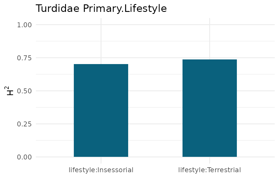

Per-contrast phylogenetic heritability, baseline category Generalist.

One categorical draw per species — read the correlation with caution, or not at all. This dataset has exactly one lifestyle observation per species, the regime the package’s own recovery campaign (documented for this exact call shape) found unreliable for the among-category correlation: variance/H^2 components separate and recover correctly, but the correlation estimate rails toward +/-1 in a substantial fraction of simulated fits under one draw per species, even with a positive-definite Hessian. Five or more independent categorical draws per species resolves it in simulation; a real comparative dataset with one row per species — like this one — cannot supply that, so this article reports the per-contrast H^2 values above and does not report or interpret a phylogenetic correlation between lifestyle categories.

Comparison with the paper’s route

The paper fits both examples with MCMCglmm (and brms); we do not have access to its published posterior numbers and do not reproduce them here — inventing or approximating a number attributed to a published paper would be worse than not comparing at all.

For Example 1, we instead ran our own independent MCMCglmm comparator on the same data, as a second opinion rather than a validation of the paper’s own posterior:

d1$value_f <- factor(as.integer(d1$Migration_ordered), ordered = TRUE)
Ainv <- MCMCglmm::inverseA(ex1$tree, nodes = "TIPS")$Ainv
prior <- list(R = list(V = 1, fix = 1),
              G = list(G1 = list(V = 1, nu = 1, alpha.mu = 0, alpha.V = 1000)))
t0 <- Sys.time()
m <- MCMCglmm::MCMCglmm(
  value_f ~ logMass, random = ~ species, ginverse = list(species = Ainv),
  data = d1, family = "ordinal", prior = prior,
  nitt = 33000, burnin = 3000, thin = 30, verbose = FALSE
)
mcmc_wall <- as.numeric(difftime(Sys.time(), t0, units = "secs"))
h2_mcmc <- mean(m$VCV[, "species"] / (m$VCV[, "species"] + m$VCV[, "units"] + 1))
cat("MCMCglmm wall clock:", round(mcmc_wall, 1), "s\n")
cat("gllvmTMB  H2(migration), joint bivariate fit:",
    round(ps1$H2[ps1$trait == "migration"], 3), "\n")
cat("MCMCglmm  H2(migration), univariate fit:     ", round(h2_mcmc, 3), "\n")

The two numbers are not a like-for-like comparison — MCMCglmm here fits Migration_ordered alone, while gllvmTMB’s number comes from the joint bivariate fit with Habitat.Density — so read this as a qualitative sanity check, not an equivalence test. They land close (within ~0.02 on this dataset), which is reassuring but is a single comparison on one dataset, not a calibration result.

For Example 2 (nominal), no comparator is run here: MCMCglmm’s categorical family needs a from-scratch multi-trait link-function setup distinct from the ordinal case above, and building that correctly is outside this article’s scope. The comparison for Example 2 is qualitative only — read the paper directly for its own numbers.

The paper-equation to gllvmTMB-call map

The rows below map the paper’s equations to the gllvmTMB calls used in this article.

Paper eq	Model	gllvmTMB call	Status
1-5	Univariate continuous PMM	phylo_indep(0 + trait \| species, tree = tree), family = gaussian()	supported for T >= 2 traits; a genuinely univariate fit is out of scope (see above)
6-11	Multivariate PMM, Kronecker Sigma_a %x% A	phylo_dep(0 + trait \| species, tree = tree)	supported; used in Example 1 above
27-32	Ordinal PGLMM with phylogenetic source	phylo_latent() / phylo_indep() / phylo_dep() + family = ordinal_probit()	supported; used in Example 1 above
33-37	Nominal PGLMM, per-contrast phylogenetic variances/correlations	phylo_latent(species, tree = tree, d = K - 1) + family = multinomial()	supported for variance/H^2 components; the among-category correlation needs n_rep >= 5 draws per species, which single-observation comparative data does not have (Example 2 above)
4, 18, 19	Phylogenetic heritability H^2 = sigma_a^2 / (sigma_a^2 + sigma_e^2)	extract_phylo_signal(fit, link_residual = "auto")	supported; sigma_e^2 = 1 for ordinal (eq 18), pi^2/3 per contrast for nominal (eq 19), never collapsed to a scalar
8	Phylogenetic correlation between traits/contrasts	extract_correlations(fit, tier = "phy")	supported for admitted phylogenetic tiers, including ordinal and multinomial
A.1-A.9	Contrast-matrix reparameterisation of the softmax	n/a	no action needed — gllvmTMB already fits the equivalent baseline-category-logit softmax directly

The status column states the supported scope directly. Combinations not listed here should not be inferred from a neighbouring supported model.

What this article does not claim

• No calibrated interval. Cutpoint standard errors above are Wald approximations reported descriptively; no coverage study backs any interval in this article.
• gllvmTMB is a multivariate engine. A strictly univariate model — one categorical trait, no second trait to stack against it — is outside gllvmTMB’s scope; use glmmTMB or the paper’s own MCMCglmm/brms route for that case directly.
• The Example 2 phylogenetic correlation is withheld, not just under-powered. With one categorical draw per species, the correlation estimate is known to be unreliable even when the fit reports full convergence; do not read the H^2 values above as implying a trustworthy correlation exists alongside them.
• This is one dataset each, fitted once. Point estimates describe these specific fits; they are not simulation-based recovery evidence.
• No ancestral-state reconstruction. The paper’s Bayesian route supports this; gllvmTMB does not attempt it.

See also

• Phylogenetic covariance among traits — the continuous-trait phylogenetic GLLVM this article’s ordinal/nominal models build on.
• Unordered categories with multinomial() — the general nominal-response guide.
• Choose a response family — when to reach for ordinal_probit() vs multinomial() vs binomial().