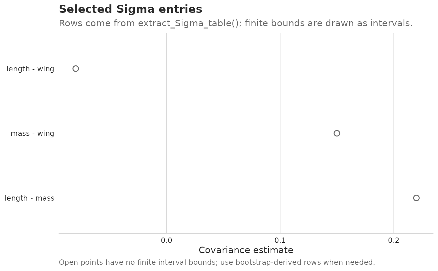
plot_Sigma_table() turns rows from extract_Sigma_table() into a
forest-style covariance or correlation plot. It is designed for reports and
articles that need to show selected covariance entries without indexing the
Sigma matrix by hand. Rows without finite interval bounds are drawn as
open points. To display Sigma uncertainty, pass interval-bearing rows, for
example from a bootstrap workflow; extract_Sigma_table() itself currently
leaves interval columns as placeholders.
Usage
plot_Sigma_table(
  x,
  level = "unit",
  part = c("total", "shared", "unique"),
  measure = c("covariance", "correlation"),
  entries = c("upper", "unique", "all", "offdiag", "lower", "diag"),
  link_residual = c("auto", "none"),
  include_diagonal = FALSE,
  facet = c("level", "none"),
  sort = c("estimate", "magnitude", "trait", "level"),
  show_intervals = NULL,
  style = c("interval", "eye", "raindrop"),
  eye_level = 0.95,
  raindrop_level = NULL
)
Arguments
- x
A fit returned by
gllvmTMB(), an admittedengine = "julia"bridge fit, abootstrap_Sigmaobject, or a data frame returned byextract_Sigma_table(). Data frames must containlevel,trait_i,trait_j,estimate,lower,upper,matrix,component,diagonal, andtriangle.- level, part, measure, entries, link_residual
Passed to
extract_Sigma_table()whenxis a fitted model. The plotting defaultentries = "upper"shows each pairwise covariance/correlation once; passentries = "diag"for variances orentries = "unique"for the diagonal plus upper triangle.- include_diagonal
Logical. Include diagonal rows if they are present in
x? The default isFALSEbecause covariance diagonals are variances and are usually on a different interpretive scale than pairwise covariances.- facet
One of
"level"(default) or"none".- sort
Row ordering:
"estimate"(default),"magnitude","trait", or"level".- show_intervals
Logical or
NULL. IfNULL(default), finitelower/upperbounds are drawn as horizontal intervals forstyle = "interval"and omitted forstyle = "eye". SetTRUEto overlay interval lines on confidence eyes. Rows without finite bounds remain visible as points.- style
One of
"interval"(default),"eye", or"raindrop"."eye"draws a confidence eye: a pale frequentist compatibility shape reconstructed from the estimate and finite interval bounds, plus a hollow, sign-coloured estimate circle. Correlation rows use Fisher's z scale and covariance rows use the displayed estimate scale. The shape is not a posterior density."raindrop"is accepted as a compatibility alias.- eye_level
Confidence level represented by the supplied interval bounds when
style = "eye". Default0.95.- raindrop_level
Compatibility alias for
eye_level.
Details
Scope: the helper plots point-estimate rows from
extract_Sigma_table() or extracts those rows from a fit returned by
gllvmTMB() or an admitted engine = "julia" bridge fit (covered by the
package's extractor-contract validation tests, including the Julia-bridge
fit path). Interval columns are displayed when present and
finite, but this helper does not compute Sigma intervals.
Uncertainty propagation for arbitrary Sigma entries belongs in
bootstrap/profile infrastructure.
Examples
if (requireNamespace("ggplot2", quietly = TRUE)) {
  sigma_rows <- data.frame(
    level = "unit",
    trait_i = c("length", "length", "mass"),
    trait_j = c("mass", "wing", "wing"),
    estimate = c(0.22, -0.08, 0.15),
    lower = NA_real_,
    upper = NA_real_,
    matrix = "Sigma",
    component = "total",
    diagonal = FALSE,
    triangle = "upper"
  )
  plot_Sigma_table(sigma_rows)
}