Distributional outputs and adequacy

A fitted mu formula answers “what is the expected response, given the covariates?” It does not answer two other questions an applied paper usually needs: “did I model the whole conditional distribution, not just its average?” and “how extreme, or how likely to exceed a threshold, is this observation for its covariates?” A model can have a perfectly reasonable mean structure and still misrepresent the spread, tails, or boundary behaviour of the response – and coefficients alone never reveal that. This article follows the check_drm() step in the post-fit workflow described in Checking and using fitted models.

This article covers drmTMB’s distributional-output and adequacy layer, built on one shared foundation: every fitted family exposes its own density, CDF, and quantile function at the fitted parameters (fitted_distribution()). Two families of outputs are built on it:

• Adequacy diagnostics – residuals(fit, type = "quantile"), worm_plot(), qq_plot() – randomized quantile residuals (Dunn & Smyth
  1996. that should look like a standard normal sample under a correctly specified fixed-effect distributional form.
• Distributional outputs – predict(fit, type = "quantile"), exceedance(), centile_chart() – conditional quantiles, exceedance probabilities, and centile curves at the fitted model.

The worked contrast below follows Fig. 4c of the GAMLSS Primer (Merder, Rigby, Stasinopoulos et al., Nature Reviews Methods Primers, 2026, 6:49): a location-only fit to heteroscedastic data looks fine on a coefficient table, but its quantile residuals bend a worm plot and fail a normality test; the matching location-scale fit is flat and passes.

Setup

set.seed(20260712)
n <- 300
x <- stats::rnorm(n)
sigma_true <- exp(0.1 + 0.9 * x)
y <- 0.3 + 0.6 * x + stats::rnorm(n, sd = sigma_true)
dat <- data.frame(y = y, x = x)

y is generated with a residual SD that grows with x: a Gaussian location-scale problem, not a location-only one.

Quantile residuals and worm/QQ plots on a correctly specified fit

Fit the model that matches the data-generating process – mu and sigma both depend on x – and compute randomized quantile residuals.

fit_true <- drmTMB(bf(y ~ x, sigma ~ x), family = gaussian(), data = dat)
r_true <- residuals(fit_true, type = "quantile")
stats::ks.test(r_true, "pnorm")
#> 
#>  Asymptotic one-sample Kolmogorov-Smirnov test
#> 
#> data:  r_true
#> D = 0.031089, p-value = 0.9339
#> alternative hypothesis: two-sided

The residuals are indistinguishable from a standard normal sample: a Kolmogorov-Smirnov test does not reject. worm_plot() (a detrended QQ plot) and qq_plot() show the same thing visually – a flat scatter around the reference line is “no detectable departure from N(0,1),” never proof the model is correct.

worm_plot(fit_true) +
  ggplot2::labs(
    subtitle = "Fixed-effect adequacy: no detectable departure from N(0,1)"
  )

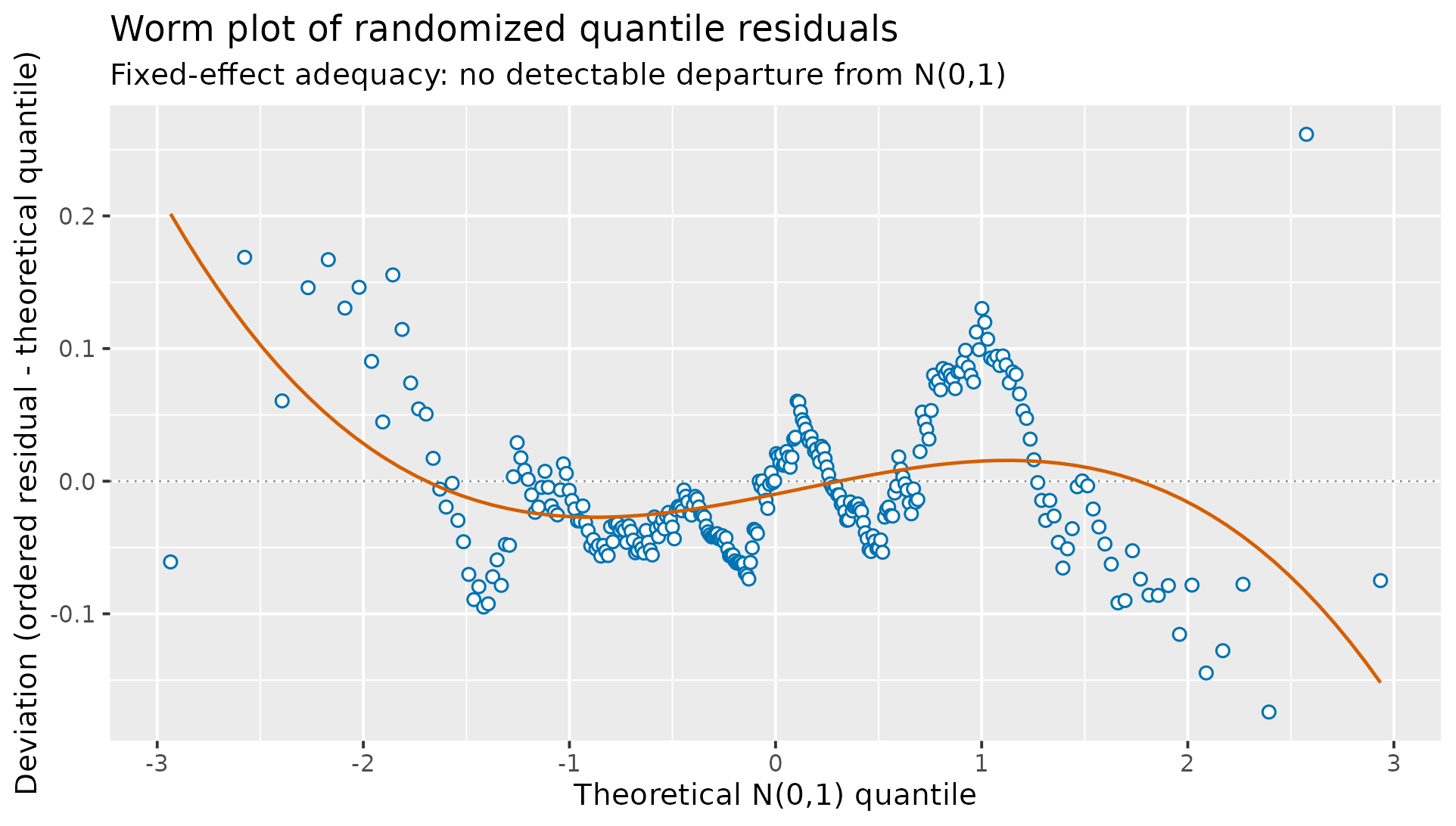
Worm plot of quantile residuals for the correctly specified location-scale fit; the smooth stays near the zero reference across the bulk, with only sparse-tail drift (the KS test does not reject).

qq_plot(fit_true)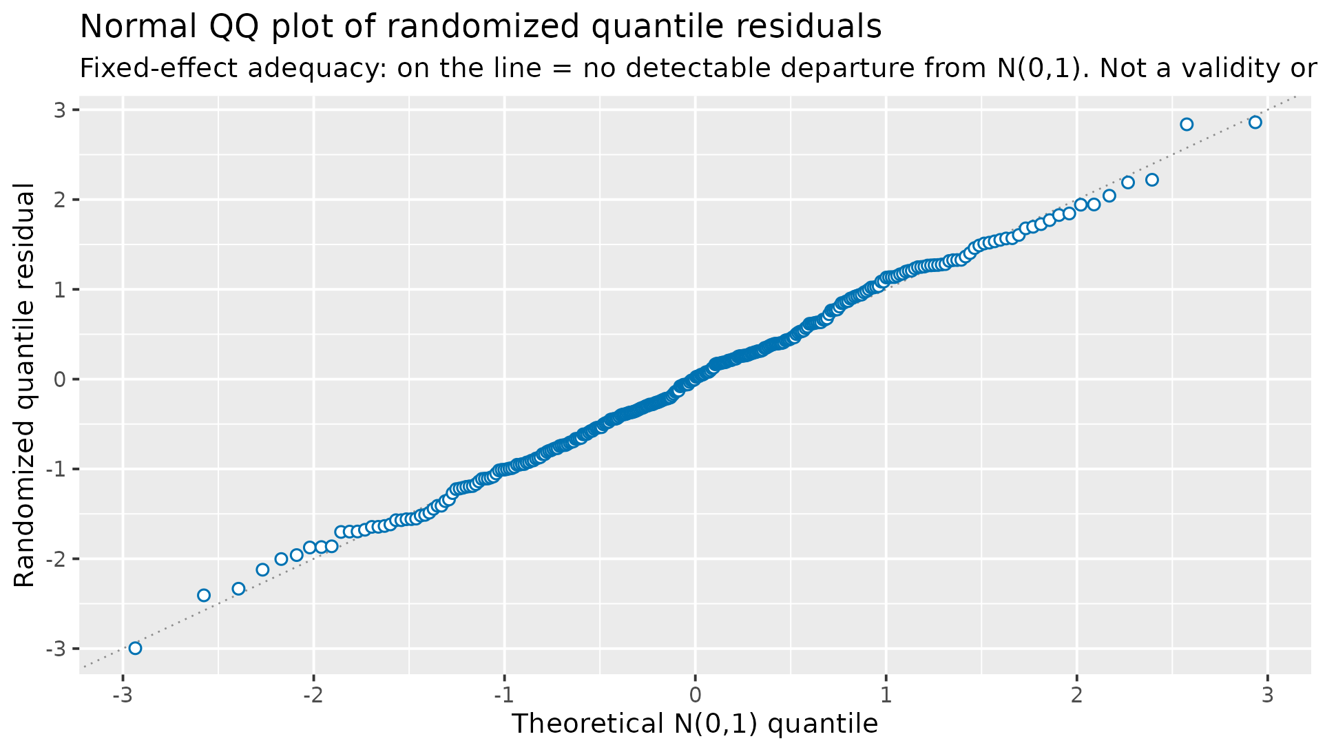

Normal QQ plot of quantile residuals for the correctly specified fit; points on the diagonal are no detectable departure from N(0,1).

Reproducing the Fig-4c contrast: a location-only fit to heteroscedastic data

Now fit a location-only model to the same data – sigma held constant, so the growing spread in y has nowhere to go but into the residuals.

fit_mis <- drmTMB(bf(y ~ x, sigma ~ 1), family = gaussian(), data = dat)
r_mis <- residuals(fit_mis, type = "quantile")
stats::ks.test(r_mis, "pnorm")
#> 
#>  Asymptotic one-sample Kolmogorov-Smirnov test
#> 
#> data:  r_mis
#> D = 0.19845, p-value = 1.093e-10
#> alternative hypothesis: two-sided

The KS test now rejects sharply. The worm plot bends into the same systematic curve the GAMLSS Primer’s Fig-4c shows: at extreme covariate values the observations are consistently too close to (or too far from) mu, because the constant sigma cannot track the true variance growth.

worm_plot(fit_mis) +
  ggplot2::labs(
    subtitle = "Fixed-effect adequacy: bend flags a detectable departure from N(0,1)"
  )

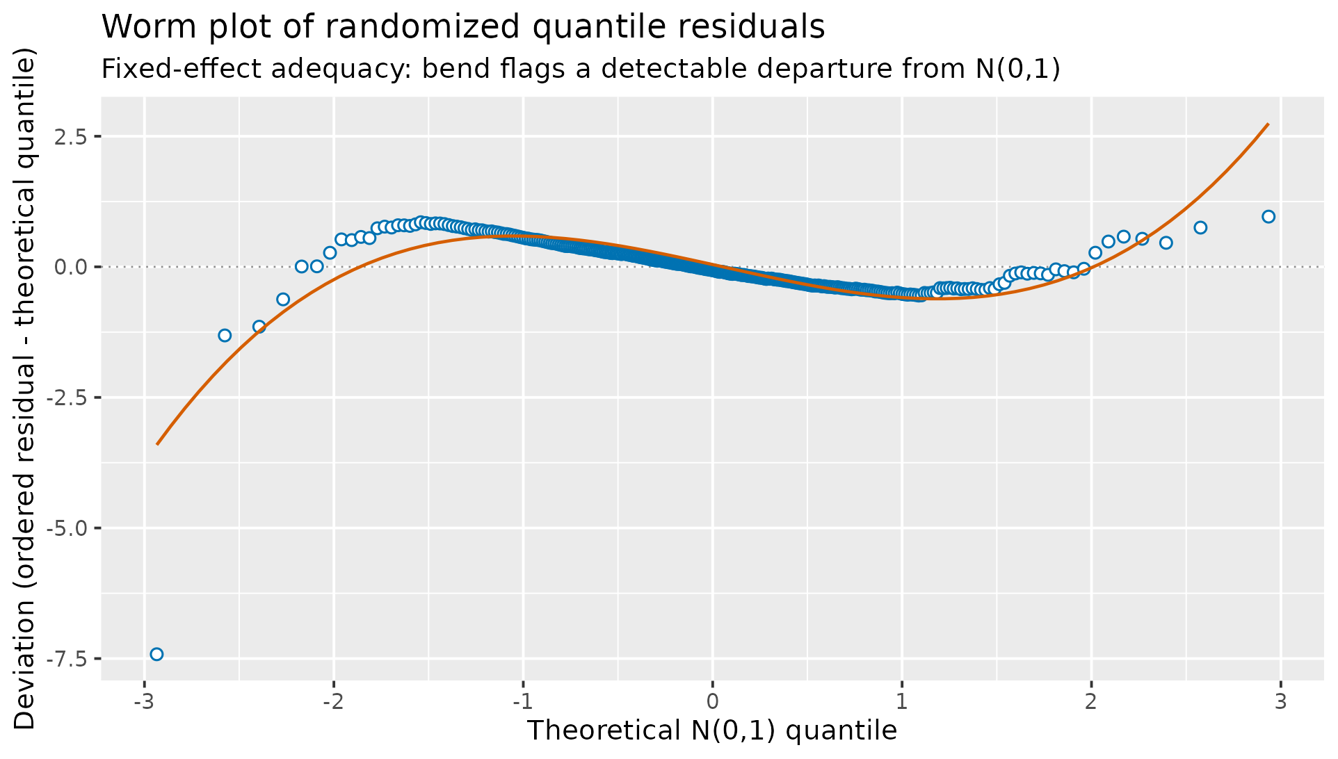
Worm plot of quantile residuals for the location-only fit to heteroscedastic data; the systematic bend flags a mis-specified distributional shape.

Both worm_plot() and qq_plot() apply this package’s Confidence-Eye figure contract: hollow points, no filled dots, no interval bars around the reference line – the reference line is a null-hypothesis benchmark, not an uncertainty interval.

The two fits have the same mu formula and produce similar coefficient tables; only the adequacy check separates them. That is the point of a distributional diagnostic: it catches a mis-specification a mean-only residual plot would miss.

Distributional outputs: quantiles, exceedance, and centiles

Beyond checking the fit, the same fitted_distribution() foundation answers conditional-quantile and threshold questions directly, using the correctly specified fit_true.

Conditional quantiles

newdata <- data.frame(x = c(-1, 0, 1))
predict(fit_true, newdata = newdata, type = "quantile", prob = c(0.025, 0.5, 0.975))
#>           2.5%        50%     97.5%
#> [1,] -1.192822 -0.2513603 0.6901018
#> [2,] -1.802150  0.3907377 2.5836249
#> [3,] -4.074916  1.0328356 6.1405873
#> attr(,"calibrated")
#> [1] FALSE
#> attr(,"prob")
#> [1] 0.025 0.500 0.975
#> attr(,"label")
#> [1] "distributional (plug-in) interval"

The output widens at extreme x because sigma grows with x in this model – exactly the heteroscedasticity the location-only fit above could not represent.

Exceedance probability

exceedance() returns Pr(Y > threshold | x) at the fitted model, a thin wrapper over the shared CDF.

exceedance(fit_true, threshold = 2, newdata = newdata)
#> [1] 1.386537e-06 7.517018e-02 3.552727e-01
#> attr(,"calibrated")
#> [1] FALSE
#> attr(,"lower.tail")
#> [1] FALSE
#> attr(,"threshold")
#> [1] 2 2 2

Centile chart

centile_chart() draws fitted response centiles against one covariate, holding every other predictor at a reference value.

centile_chart(fit_true, covariate = "x") +
  ggplot2::scale_colour_viridis_d()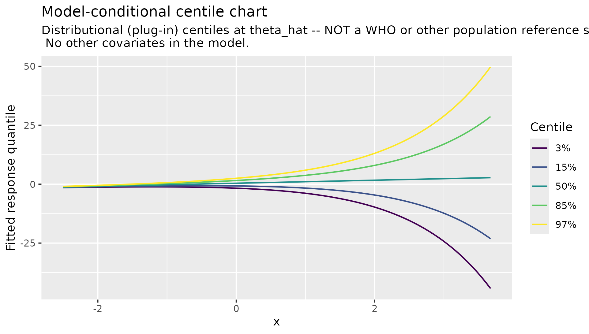

Model-conditional centile chart for the correctly specified location-scale fit; centiles fan out with x because sigma grows with x.

The centiles fan out as x increases – a direct visual reading of the fitted sigma ~ x relationship that a mean-only prediction plot would not show.

What this layer detects – and what it does not

Detects. The adequacy diagnostic reliably catches distributional shape or atom mis-specification that a family cannot reabsorb through its own free parameters: heavy tails fit as Gaussian, ignored overdispersion or zero-inflation in a family with no free dispersion parameter, ignored truncation, a missing zero/one atom, and the heteroscedasticity example reproduced above. A 400-seed gated campaign across all 18 fitted families (tweedie: 99 of 400 seeds locally, 66/99 dispersion-arm non-convergence, full run deferred to Totoro) (docs/dev-log/simulation-artifacts/2026-07-12-dg3-power-arm-gated/) confirms type-I error at or below the nominal rate under a correctly specified fit, with power >= 0.8 (commonly 0.9-1.0) for these detectable mis-specifications.

Does not detect – a structural blind spot, not evidence of adequacy. When a fitted family’s own free nuisance, dispersion, or inflation parameter can absorb a mis-specification, the marginal quantile residual stays close to N(0,1) even though the mean or variance structure is wrong. Examples from the same campaign: heteroscedasticity absorbed by Student-t nu (power 0.035, versus 1.0 for the same heteroscedasticity under Gaussian, which has no absorbing parameter); missing zero-inflation absorbed by nbinom2’s sigma (power 0.035, versus 0.96 under Poisson); and a constant-vs-covariate zero-inflation/hurdle/zero-one-inflation mechanism, which splits in two: for hurdle_nbinom2/zero_one_beta power stays flat near the type-I rate regardless of sample size (a genuine structural blind spot); for zi_poisson/zi_nbinom2 power rises with sample size but stays far below 0.8 even at n = 3000, so it is impractical to detect at realistic sample sizes rather than permanently undetectable. A mean-structure diagnostic, not this one, is what catches an absorbed mis-specification.

Wording and scope, throughout this package:

• Passing this diagnostic means “no detectable departure from N(0,1),” and is worded that way everywhere – never “the model is adequate,” “valid,” or “correct.”
• residuals(type = "quantile"), worm_plot(), and qq_plot() are fixed-effect adequacy: for a random-effect or structured fit, they are conditional on the fixed-effect prediction, not a marginal check of the full model.
• predict(type = "quantile") and exceedance() results carry attr(., "calibrated") <- FALSE: they are distributional (plug-in) outputs at the fitted parameter point estimate, and do not propagate parameter uncertainty. centile_chart() is a model-conditional curve at that same point estimate, not a WHO-style or other population reference standard.
• A distributional-output or adequacy tick never changes, or implies anything about, a family’s separate inference-tier status (see vignettes/capability-and-limits.Rmd). Fitting quantiles and residuals for a family does not certify its confidence intervals.

See docs/dev-log/known-limitations.md for the full scope note and docs/dev-log/simulation-artifacts/2026-07-12-dg3-power-arm-gated/ for the underlying campaign this section summarizes.