Changing residual coupling with rho12 • drmTMB

This tutorial introduces bivariate location-scale regression with predictor-dependent residual correlation. It assumes the univariate location-scale reading pattern from When variance carries signal and extends it to two responses. The scientific idea is that two responses can change in mean, change in residual variance, and change in residual coupling.

Current fixed-effect syntax uses one formula per distributional parameter:

drmTMB(
  drm_formula(
    mu1 = y1 ~ x1 + x2,
    mu2 = y2 ~ x1,
    sigma1 = ~ x1 + x2,
    sigma2 = ~ x1,
    rho12 = ~ x1 + x2
  ),
  family = c(gaussian(), gaussian()),
  data = dat
)

The central modelling question is whether predictors change residual coupling between two responses, not only their means or variances.

The key parameter is rho12. A location-scale model asks whether predictors change residual SDs. A location-coscale model asks whether predictors also change the residual covariance structure between two responses; in the current bivariate Gaussian model, that structure is the residual correlation rho12. In ecology and evolution, this can ask whether the residual association between traits such as body mass and litter size differs among terrestrial, aquatic, and aerial lifestyles after modelling response-specific means and dispersion.

Equations for the implemented model

For observation i, the implemented fixed-effect bivariate Gaussian model is:

$\begin{bmatrix} y_{1i} \\ y_{2i} \end{bmatrix} \mid \mu_{1i}, \mu_{2i}, \sigma_{1i}, \sigma_{2i}, \rho_{12i} \sim \operatorname{MVN} \left( \begin{bmatrix} \mu_{1i} \\ \mu_{2i} \end{bmatrix}, \Omega_i \right).$

The five distributional predictors are:

$\begin{aligned} \mu_{1i} &= X_{\mu 1,i}\beta_{\mu 1}, \\ \mu_{2i} &= X_{\mu 2,i}\beta_{\mu 2}, \\ \log(\sigma_{1i}) &= X_{\sigma 1,i}\beta_{\sigma 1}, \\ \log(\sigma_{2i}) &= X_{\sigma 2,i}\beta_{\sigma 2}, \\ \eta_{\rho12,i} &= X_{\rho12,i}\beta_{\rho12}, \\ \rho_{12i} &= \tanh(\eta_{\rho12,i}). \end{aligned}$

The residual covariance matrix is:

$\Omega_i = \begin{bmatrix} \sigma_{1i}^2 & \rho_{12i}\sigma_{1i}\sigma_{2i} \\ \rho_{12i}\sigma_{1i}\sigma_{2i} & \sigma_{2i}^2 \end{bmatrix}.$

Component meanings:

Component	Meaning
`mu1`, `mu2`	expected values for responses 1 and 2
`sigma1`, `sigma2`	residual SDs for responses 1 and 2
`eta_rho12`	unconstrained linear predictor for residual correlation
`rho12`	residual response-response correlation within observation `i`
`Omega_i`	residual covariance matrix after means and residual SDs are modelled

For implementation cross-checking, the same model can also be written in a compact code-like form:

mu1_i = X_mu1[i, ] beta_mu1
mu2_i = X_mu2[i, ] beta_mu2
log(sigma1_i) = X_sigma1[i, ] beta_sigma1
log(sigma2_i) = X_sigma2[i, ] beta_sigma2
eta_rho12_i = X_rho12[i, ] beta_rho12
rho12_i = tanh(eta_rho12_i)
Omega_i[1, 1] = sigma1_i^2
Omega_i[2, 2] = sigma2_i^2
Omega_i[1, 2] = Omega_i[2, 1] = rho12_i * sigma1_i * sigma2_i

Implementation note: drmTMB internally evaluates residual correlations as 0.999999 * tanh(eta_rho12_i). The tiny multiplier keeps covariance matrices strictly positive definite near the boundaries. It is not a biological scaling factor, and it should not change how users interpret the model.

The matching drmTMB syntax is:

drmTMB(
  bf(
    mu1 = y1 ~ x1 + x2,
    mu2 = y2 ~ x1,
    sigma1 = ~ x1 + x2,
    sigma2 = ~ x1,
    rho12 = ~ x1 + x2
  ),
  family = c(gaussian(), gaussian()),
  data = dat
)

The mapping is:

Symbol	Meaning	R syntax source
`y1_i`, `y2_i`	observed responses	left-hand sides of `mu1` and `mu2` formulas
`X_mu1`, `X_mu2`	response-specific mean design matrices	right-hand sides of `mu1` and `mu2`
`mu1_i`, `mu2_i`	fitted response-specific means	columns of `fitted(fit)`
`X_sigma1`, `X_sigma2`	response-specific residual scale design matrices	right-hand sides of `sigma1` and `sigma2`
`X_rho12`	residual correlation design matrix	right-hand side of `rho12`
`sigma1_i`, `sigma2_i`	residual SDs for responses 1 and 2	`predict(fit, dpar = "sigma1")`, `predict(fit, dpar = "sigma2")`
`rho12_i`	residual response-response correlation	`rho12(fit)`

The fixed effects may be the same, overlapping, or different across parameters. For example, x1 can appear in all five formulae, while x2 might appear only in mu1, sigma1, and rho12. Each parameter still gets its own coefficient vector.

Read those coefficient vectors as separate biological statements:

Formula	Example coefficient	Interpretation
`mu1 = y1 ~ x`	`mu1:x`	predictor effect on the expected value of response 1
`mu2 = y2 ~ x`	`mu2:x`	predictor effect on the expected value of response 2
`sigma1 = ~ x`	`sigma1:x`	multiplicative change in residual SD for response 1
`sigma2 = ~ x`	`sigma2:x`	multiplicative change in residual SD for response 2
`rho12 = ~ x`	`rho12:x`	change in residual response-response coupling after both means and residual SDs are modelled

The rho12 slope is not a slope for either response mean. It is a slope on the correlation-link scale. Use rho12(fit, newdata = grid) or a rho12 curve when the reader needs the fitted residual correlation on the response scale.

If both responses have the same location predictors, mvbind() is a shorthand for the two location formulas:

drmTMB(
  bf(
    mvbind(y1, y2) ~ x1 + x2,
    sigma1 = ~ x1 + x2,
    sigma2 = ~ x1,
    rho12 = ~ x1 + x2
  ),
  family = c(gaussian(), gaussian()),
  data = dat
)

This expands internally to mu1 = y1 ~ x1 + x2 and mu2 = y2 ~ x1 + x2. Use explicit mu1 and mu2 formulas whenever the responses need different location predictors.

Worked example: behaviour coupling and disturbance

Suppose an ecologist measures two behaviours, activity and boldness, and wants to know whether an environmental gradient changes their residual coupling after accounting for response-specific means and residual SDs. The code below uses simulated data, but the model structure matches that scientific question.

For this example, the fitted biological model is:

$\begin{aligned} \begin{bmatrix} \text{activity}_i\\ \text{boldness}_i \end{bmatrix} &\sim \operatorname{MVN} \left( \begin{bmatrix} \mu_{\text{activity},i}\\ \mu_{\text{boldness},i} \end{bmatrix}, \Omega_i \right),\\ \mu_{\text{activity},i} &= \beta_{a0} + \beta_{a1}\text{food}_i + \beta_{a2}\text{temperature}_i,\\ \mu_{\text{boldness},i} &= \beta_{b0} + \beta_{b1}\text{food}_i,\\ \log(\sigma_{\text{activity},i}) &= \gamma_{a0} + \gamma_{a1}\text{food}_i + \gamma_{a2}\text{temperature}_i,\\ \log(\sigma_{\text{boldness},i}) &= \gamma_{b0} + \gamma_{b1}\text{food}_i,\\ \eta_{\rho12,i} &= \delta_0 + \delta_1\text{disturbance}_i,\\ \rho_{12,i} &= \tanh(\eta_{\rho12,i}). \end{aligned}$

Here rho12 is not the ordinary correlation between raw activity and raw boldness. It is the residual correlation after the model has already adjusted for the mean and residual SD predictors in each response.

set.seed(1)
n <- 180
dat <- data.frame(
  food = rnorm(n),
  temperature = rnorm(n),
  disturbance = rnorm(n)
)
mu1 <- 0.2 + 0.5 * dat$food + 0.2 * dat$temperature
mu2 <- -0.1 + 0.4 * dat$food
sigma1 <- exp(-0.2 + 0.2 * dat$food - 0.1 * dat$temperature)
sigma2 <- exp(0.1 - 0.2 * dat$food)
eta_rho12 <- -0.1 + 0.4 * dat$disturbance
rho12 <- tanh(eta_rho12)
e1 <- rnorm(n)
e2 <- rho12 * e1 + sqrt(1 - rho12^2) * rnorm(n)
dat$activity <- mu1 + sigma1 * e1
dat$boldness <- mu2 + sigma2 * e2

The model lets food and temperature explain mean activity, lets food explain mean boldness, lets food and temperature explain residual SD in activity, lets food explain residual SD in boldness, and lets disturbance explain residual correlation:

fit_biv <- drmTMB(
  drm_formula(
    mu1 = activity ~ food + temperature,
    mu2 = boldness ~ food,
    sigma1 = ~ food + temperature,
    sigma2 = ~ food,
    rho12 = ~ disturbance
  ),
  family = c(gaussian(), gaussian()),
  data = dat
)

Check the fit and inspect the coefficient table:

check_drm(fit_biv)
#> <drm_check: 13 checks>
#> ok: 12; notes: 0; warnings: 1; errors: 0
#>                      check  status
#>      optimizer_convergence      ok
#>           optimizer_budget      ok
#>           finite_objective      ok
#>      logsigma_clamp_active      ok
#>             fixed_gradient warning
#>            sdreport_status      ok
#>  hessian_positive_definite      ok
#>     standard_errors_finite      ok
#>   standard_errors_inflated      ok
#>               dropped_rows      ok
#>             positive_scale      ok
#>             rho12_boundary      ok
#>   fixed_effect_design_size      ok
#>                                                                                   value
#>                                                                                       0
#>                                                 iterations=19; function=30; gradient=19
#>                                                                                   495.7
#>                                                                                    <NA>
#>                                                  max=0.001030; component=beta_sigma2[1]
#>                                                                                      ok
#>                                                                                    TRUE
#>                                                                 range=[0.05053,0.08091]
#>                                         n_inflated=0; max_se=0.08091; median_se=0.05655
#>                                                                     nobs=180; dropped=0
#>                                                                              min=0.5408
#>                                                                                  0.9633
#>  total_mb=0.07536; max_cols=3; largest=mu1; largest_class=matrix; largest_density=1.000
#>                                                                              message
#>                                                        nlminb convergence code is 0.
#>  Optimizer evaluation counts recorded; no eval.max or iter.max control was supplied.
#>                                             Objective and log-likelihood are finite.
#>                                   The log(sigma) clamp is not active at the optimum.
#>     Maximum absolute fixed gradient is > 0.001; largest component is beta_sigma2[1].
#>                                              TMB::sdreport() completed successfully.
#>                                        sdreport reports a positive-definite Hessian.
#>                                         All fixed-effect standard errors are finite.
#>                   No fixed-effect standard error is inflated relative to the others.
#>                   No rows were dropped by model-frame or known-covariance filtering.
#>                                     All fitted scale values are finite and positive.
#>                        All fitted residual correlations have absolute value <= 0.98.
#>                          Dense fixed-effect design matrices are modest for this fit.
summary(fit_biv)
#> <summary.drmTMB>
#> estimator: ML
#>                        estimate  std_error
#> mu1:(Intercept)     0.130704577 0.05416604
#> mu1:food            0.565333676 0.06286358
#> mu1:temperature     0.217923280 0.05437145
#> mu2:(Intercept)    -0.081403393 0.07949003
#> mu2:food            0.330436681 0.08090972
#> sigma1:(Intercept) -0.155134470 0.05052618
#> sigma1:food         0.208912661 0.05454887
#> sigma1:temperature  0.003850637 0.05566011
#> sigma2:(Intercept)  0.209289411 0.05234188
#> sigma2:food        -0.192522639 0.05744758
#> rho12:(Intercept)  -0.004442462 0.07014734
#> rho12:disturbance   0.523480411 0.06355325
#> Distributional, random-effect, scale, and correlation parameters:
#>                          component   dpar         term   estimate    minimum
#> fitted:sigma1 distributional-scale sigma1 fitted range  0.8834355  0.5408486
#> fitted:sigma2 distributional-scale sigma2 fitted range  1.2386315  0.7764086
#> fitted:rho12  residual-correlation  rho12 fitted range -0.0254550 -0.9184598
#>                maximum    scale
#> fitted:sigma1 1.418099 response
#> fitted:sigma2 1.888286 response
#> fitted:rho12  0.963325 response
#> logLik: -495.7
#> convergence: 0

How to read this output:

Rows beginning with mu1: describe expected activity, and rows beginning with mu2: describe expected boldness.
Rows beginning with sigma1: and sigma2: describe log residual SDs for activity and boldness.
Rows beginning with rho12: describe the residual activity-boldness correlation on the linear-predictor scale. Use rho12(fit_biv) or rho12(fit_biv, newdata = ...) to read that effect as a correlation.

The rho12 coefficients are on the linear-predictor scale:

coef(fit_biv, "rho12")
#>  (Intercept)  disturbance 
#> -0.004442462  0.523480411
head(rho12(fit_biv))
#> [1] -0.87673390  0.59373244 -0.32491851 -0.22558016 -0.09280934  0.30592318

corpairs() gives the same residual correlation in the long correlation-pair format. The same table shape now also holds fitted ordinary group-level and structured rows where their covariance routes are fitted, including phylogenetic, coordinate-spatial, animal-model, and relmat() q=2 or constant q=4 rows. Predictor-dependent spatial, animal, relmat(), study-level, q=4, residual-scale, and slope-specific corpair() regressions remain planned:

corpairs(fit_biv)[
  c("level", "from_response", "to_response", "class", "parameter",
    "estimate", "min", "max", "modelled")
]
#>      level from_response to_response    class parameter  estimate        min
#> 1 residual      activity    boldness residual     rho12 -0.025455 -0.9184598
#>        max modelled
#> 1 0.963325     TRUE

The rho12 coefficients are fitted on the linear-predictor scale eta_rho12; the response transform is rho12 = tanh(eta_rho12) with the tiny internal guard described above. Use rho12(fit) to read them as residual correlations, and use corpairs(fit) to place residual rho12 in a table that is ready to hold other correlation levels later. In this example, a positive coefficient for disturbance means that observations with larger disturbance have stronger positive residual coupling between activity and boldness, after the model has already accounted for the predictors in mu1, mu2, sigma1, and sigma2.

Keep the three correlation words separate:

Word	Use it for	Do not use it for
`rho12`	the residual bivariate Gaussian coscale formula and extractor	group-level, phylogenetic, spatial, animal-model, or known-matrix covariance
`corpair()`	a formula for an implemented predictor-dependent latent random-effect pair, currently selected q=2 ordinary and phylogenetic location-location routes	residual correlation or q=4, spatial, animal, `relmat()`, residual-scale, and slope-specific correlation regressions
`corpairs()`	extracting fitted residual and latent correlation rows from the model object	asking the model to fit a new covariance structure

A location-scale model changes sigma; a location-coscale model changes residual rho12. A double-hierarchical or structured covariance model may also report latent correlations through corpairs(), but those rows answer questions about group, phylogenetic, spatial, animal-model, or known-matrix deviations rather than residual coupling within an observation.

newdat <- data.frame(
  food = 0,
  temperature = 0,
  disturbance = c(-1, 0, 1)
)
rho_table <- data.frame(
  disturbance = newdat$disturbance,
  sigma_activity = predict(fit_biv, newdata = newdat, dpar = "sigma1"),
  sigma_boldness = predict(fit_biv, newdata = newdat, dpar = "sigma2"),
  rho12 = rho12(fit_biv, newdata = newdat)
)
rho_table$residual_covariance <- with(
  rho_table,
  rho12 * sigma_activity * sigma_boldness
)
rho_table$residual_variance_activity <- rho_table$sigma_activity^2
rho_table$residual_variance_boldness <- rho_table$sigma_boldness^2
round(rho_table, 3)
#>   disturbance sigma_activity sigma_boldness  rho12 residual_covariance
#> 1          -1          0.856          1.233 -0.484              -0.511
#> 2           0          0.856          1.233 -0.004              -0.005
#> 3           1          0.856          1.233  0.477               0.503
#>   residual_variance_activity residual_variance_boldness
#> 1                      0.733                       1.52
#> 2                      0.733                       1.52
#> 3                      0.733                       1.52

This table gives three quantities a reader can report directly. sigma_activity and sigma_boldness are the fitted residual SDs for each response at the chosen covariate values. rho12 is the fitted residual correlation between the two responses. residual_covariance is the off-diagonal element of \Omega_i, computed as rho12 * sigma_activity * sigma_boldness. The two residual variance columns are the diagonal elements of \Omega_i.

What should I report?

For a location-coscale model, a useful result sentence usually needs all three distributional pieces: means, residual SDs, and residual coupling. A minimal table for the coscale part is:

report_grid <- data.frame(
  food = 0,
  temperature = 0,
  disturbance = c(-1.5, 0, 1.5)
)
report_table <- data.frame(
  disturbance = report_grid$disturbance,
  eta_rho12 = predict(
    fit_biv,
    newdata = report_grid,
    dpar = "rho12",
    type = "link"
  ),
  rho12 = rho12(fit_biv, newdata = report_grid),
  sigma_activity = predict(fit_biv, newdata = report_grid, dpar = "sigma1"),
  sigma_boldness = predict(fit_biv, newdata = report_grid, dpar = "sigma2")
)
report_table$residual_covariance <- with(
  report_table,
  rho12 * sigma_activity * sigma_boldness
)
report_table$residual_variance_activity <- report_table$sigma_activity^2
report_table$residual_variance_boldness <- report_table$sigma_boldness^2
round(report_table, 3)
#>   disturbance eta_rho12  rho12 sigma_activity sigma_boldness
#> 1        -1.5    -0.790 -0.658          0.856          1.233
#> 2         0.0    -0.004 -0.004          0.856          1.233
#> 3         1.5     0.781  0.653          0.856          1.233
#>   residual_covariance residual_variance_activity residual_variance_boldness
#> 1              -0.695                      0.733                       1.52
#> 2              -0.005                      0.733                       1.52
#> 3               0.689                      0.733                       1.52

The raw correlation between activity and boldness is not the same estimand as rho12. The raw correlation mixes mean structure, residual SDs, and residual coupling. The fitted rho12 is the residual correlation after the model has accounted for the formulae in mu1, mu2, sigma1, and sigma2:

round(data.frame(
  raw_activity_boldness_correlation = stats::cor(dat$activity, dat$boldness),
  mean_fitted_residual_rho12 = mean(rho12(fit_biv))
), 3)
#>   raw_activity_boldness_correlation mean_fitted_residual_rho12
#> 1                             0.021                     -0.025

When reporting this model, avoid saying only “activity and boldness were correlated”. A better sentence is: “After modelling response-specific means and residual SDs, the fitted residual activity-boldness correlation increased with disturbance.” That sentence tells the reader which correlation has been modelled.

The same response-scale result can be visualised as a rho12 curve. Here the ribbon is a 95% Wald interval from predict_parameters(). A predictor-dependent rho12 has no single scalar target, so you must supply newdata and the interval is computed for each supplied row; confint(..., parm = "rho12", newdata = ..., method = "profile") gives the profile counterpart. Treat both as computed but not coverage-certified: no simulation study yet establishes their nominal coverage for a regression rho12. Fit rho12 ~ 1 when you want the constant residual-correlation profile interval. That interval is finite and can be reported, but its coverage is not certified either: the current ledger has no committed bivariate fixed-effect CI-coverage study for this constant rho12 cell.

rho_grid <- data.frame(
  food = 0,
  temperature = 0,
  disturbance = seq(-2, 2, length.out = 80)
)
rho_pred <- predict_parameters(
  fit_biv,
  newdata = rho_grid,
  dpar = "rho12",
  conf.int = TRUE
)
rho_grid$rho12 <- rho_pred$estimate
rho_grid$conf.low <- rho_pred$conf.low
rho_grid$conf.high <- rho_pred$conf.high

if (requireNamespace("ggplot2", quietly = TRUE)) {
  ggplot2::ggplot(rho_grid, ggplot2::aes(disturbance, rho12)) +
    ggplot2::geom_hline(yintercept = 0, linetype = "dotted", colour = "grey60") +
    ggplot2::geom_ribbon(
      ggplot2::aes(ymin = conf.low, ymax = conf.high),
      fill = "#006D77",
      alpha = 0.18,
      colour = NA
    ) +
    ggplot2::geom_line(linewidth = 0.9, colour = "#006D77") +
    ggplot2::coord_cartesian(ylim = c(-1, 1)) +
    ggplot2::labs(
      x = "Disturbance",
      y = "Fitted residual correlation (rho12)",
      title = "Residual coupling changes with disturbance",
      subtitle = "Ribbon is a 95% Wald interval; dotted line marks rho12 = 0"
    ) +
    ggplot2::theme_minimal(base_size = 11) +
    ggplot2::theme(
      panel.grid.minor = ggplot2::element_blank(),
      plot.title = ggplot2::element_text(face = "bold"),
      plot.subtitle = ggplot2::element_text(colour = "grey30"),
      plot.background = ggplot2::element_rect(fill = "white", colour = NA),
      panel.background = ggplot2::element_rect(fill = "white", colour = NA)
    )
} else {
  old_par <- graphics::par(bg = "white")
  on.exit(graphics::par(old_par), add = TRUE)
  plot(
    rho12 ~ disturbance,
    data = rho_grid,
    type = "l",
    lwd = 2,
    ylim = c(-1, 1),
    xlab = "Disturbance",
    ylab = "Fitted residual correlation (rho12)"
  )
  abline(h = 0, lty = 3, col = "grey60")
}

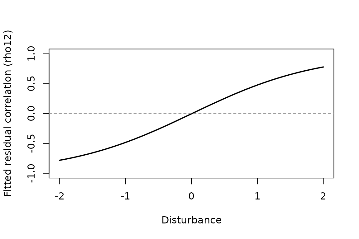
Line plot of fitted residual rho12 correlation over disturbance with a pale 95 percent Wald confidence ribbon and a dotted zero line, increasing from negative to positive values and crossing zero near average disturbance.

Fitted residual rho12 over disturbance after modelling response-specific means and residual SDs; the ribbon is a 95% Wald confidence interval computed for each supplied row (coverage not certified) and the dotted line marks zero residual correlation.

In this example, a positive disturbance coefficient for rho12 means that activity and boldness become more tightly positively coupled at higher disturbance, after their means and residual SDs have been modelled. It does not say that disturbance changes among-individual personality or plasticity correlations; those require group-level covariance blocks and should appear as separate rows in corpairs(fit).

A concise reporting sentence would be: after accounting for food, temperature, and response-specific residual SDs, the fitted residual correlation between activity and boldness increased along the disturbance gradient. In biological terms, individuals that were more active than expected were also more bold than expected under higher disturbance.

Where residual rho12 stops

The fitted model above has no repeated-individual structure. It estimates residual coupling: whether two measurements from the same observation are closer together or farther apart than expected after modelling their means and residual SDs. That is useful, but it is not the same question as whether some individuals have consistently high activity and consistently high boldness.

For ecological and evolutionary examples, residual rho12 can represent changing residual coupling between traits such as activity and boldness, body size and fecundity, or leaf area and seed number. A group-level covariance block asks a different question: do groups, individuals, species, or sites share latent deviations across fitted components?

Worked example: individual differences

Suppose the same ecologist repeatedly measures each individual and now asks an individual-difference question. After accounting for food and disturbance, do individuals with higher average activity also tend to have higher average boldness?

The first fitted group-level version adds matching labelled random intercepts in the mean structure. The shared p label creates one covariance block for the mu1 and mu2 random intercepts:

drmTMB(
  formula = bf(
    mu1 = activity ~ food + disturbance + (1 | p | ID),
    mu2 = boldness ~ food              + (1 | p | ID),
    sigma1 = ~1,
    sigma2 = ~1,
    rho12 = ~1,
    corpair(ID, level = "group", block = "p", from = "mu1", to = "mu2") ~ 1
  ),
  family = biv_gaussian(),
  data = dat_group
)

Here sigma1 and sigma2 are residual scale parameters. The fitted random-intercept SDs are group-level standard deviations in sdpars$mu, not residual sigma.

Symbolically, the implemented random-intercept mean part is:

$\begin{aligned} \mu_{1ij} &= X_{\mu 1}[ij, ]\beta_{\mu 1} + b_{0,1j},\\ \mu_{2ij} &= X_{\mu 2}[ij, ]\beta_{\mu 2} + b_{0,2j},\\ \begin{bmatrix} b_{0,1j}\\ b_{0,2j} \end{bmatrix} &\sim \operatorname{MVN}(\mathbf{0}, \Sigma_{\mu,ID}). \end{aligned}$

The covariance matrix Sigma_mu_ID contains two group-level standard deviations and one group-level correlation. That correlation answers whether individuals with higher average activity also tend to have higher average boldness. It is not rho12_i. The parameter rho12_i remains the observation-level residual correlation in Omega_i.

The small simulation below creates repeated observations from that model:

set.seed(98)
n_ID <- 55
n_each <- 7
ID <- factor(rep(seq_len(n_ID), each = n_each))
id_index <- as.integer(ID)
n <- length(ID)

food <- rnorm(n)
disturbance <- rnorm(n)

sigma_activity <- 0.35
sigma_boldness <- 0.45
sd_activity_ID <- 0.65
sd_boldness_ID <- 0.65
rho_ID <- 0.55
rho_residual <- 0.15

u_activity <- rnorm(n_ID)
u_boldness <- rho_ID * u_activity + sqrt(1 - rho_ID^2) * rnorm(n_ID)

e_activity <- rnorm(n)
e_boldness <- rho_residual * e_activity +
  sqrt(1 - rho_residual^2) * rnorm(n)

dat_group <- data.frame(ID = ID, food = food, disturbance = disturbance)
dat_group$activity <- 0.25 + 0.45 * food + 0.15 * disturbance +
  sd_activity_ID * u_activity[id_index] + sigma_activity * e_activity
dat_group$boldness <- -0.15 + 0.35 * food +
  sd_boldness_ID * u_boldness[id_index] + sigma_boldness * e_boldness

Fit the grouped model with matching (1 | p | ID) terms in the two location formulas:

fit_group <- drmTMB(
  bf(
    mu1 = activity ~ food + disturbance + (1 | p | ID),
    mu2 = boldness ~ food + (1 | p | ID),
    sigma1 = ~1,
    sigma2 = ~1,
    rho12 = ~1,
    corpair(ID, level = "group", block = "p", from = "mu1", to = "mu2") ~ 1
  ),
  family = biv_gaussian(),
  data = dat_group,
  control = list(eval.max = 500, iter.max = 500)
)

In a real analysis, inspect every row of check_drm(fit_group). The filtered rows below show the convergence and covariance checks most directly tied to this individual-difference question:

group_checks <- check_drm(fit_group)
group_checks[
  group_checks$check %in% c(
    "optimizer_convergence",
    "random_effect_sd_boundary",
    "rho12_boundary",
    "biv_mu_random_effect_covariance"
  ),
  c("check", "status", "value", "message")
]
#> <drm_check: 4 checks>
#> ok: 3; notes: 1; warnings: 0; errors: 0
#>                            check status
#>            optimizer_convergence     ok
#>        random_effect_sd_boundary     ok
#>                   rho12_boundary     ok
#>  biv_mu_random_effect_covariance   note
#>                                                                                                                value
#>                                                                                                                    0
#>                                                             min=0.6263; boundary=0.0001000; term=mu.mu1:(1 | p | ID)
#>                                                                                                               0.1743
#>  class=mean-mean; rho_abs=   NA; boundary=0.9800; n_groups=55; min_group_n=7; singleton_groups=0; min_sd_ratio=1.414
#>                                                                                                                                                                                                     message
#>                                                                                                                                                                               nlminb convergence code is 0.
#>                                                                                All fitted random-effect standard deviations are finite, positive, and above the requested lower-boundary warning threshold.
#>                                                                                                                                               All fitted residual correlations have absolute value <= 0.98.
#>  The group-level correlation could not be extracted (it may be fixed via map, unmatched, or produced by a skipped sdreport). Inspect the sdreport and parameter mapping before interpreting the covariance.

Reading group-level covariance

corpairs() keeps residual and group-level correlations in the same long table without giving them the same meaning. The ordinary intercept-only q2 group row is interval-feasible but not coverage-backed, so this article keeps both rows point-only rather than presenting an unvalidated reporting interval:

pair_table <- corpairs(
  fit_group
)
pair_table[
  ,
  c(
    "level", "group", "block", "from_dpar", "to_dpar", "class",
    "parameter", "estimate", "conf.status", "interval_source", "modelled"
  )
]
#>      level group block from_dpar  to_dpar     class
#> 1 residual  <NA>  <NA>  residual residual  residual
#> 2    group    ID     p       mu1      mu2 mean-mean
#>                                       parameter  estimate   conf.status
#> 1                                         rho12 0.1743252 not_requested
#> 2 cor(mu1:(Intercept),mu2:(Intercept) | p | ID) 0.4752219 not_requested
#>   interval_source modelled
#> 1   not_available    FALSE
#> 2   not_available     TRUE

The optional plotting helper consumes that explicit table. Faceting by level keeps the residual rho12 row visually separate from the group-level random-intercept correlation:

if (requireNamespace("ggplot2", quietly = TRUE)) {
  pair_plot_table <- pair_table
  pair_plot_table$display_label <- ifelse(
    pair_plot_table$level == "residual",
    "Residual\nrho12",
    "Individual\nmean-mean"
  )
  plot_corpairs(pair_plot_table, label = "display_label", facet = NULL) +
    ggplot2::labs(
      title = "Residual and individual-level correlations are separate",
      subtitle = "Point estimates only; dotted line marks zero correlation",
      colour = NULL
    ) +
    ggplot2::theme_minimal(base_size = 11) +
    ggplot2::theme(
      panel.grid.minor = ggplot2::element_blank(),
      plot.title = ggplot2::element_text(face = "bold"),
      plot.subtitle = ggplot2::element_text(colour = "grey30"),
      legend.position = "none"
    )
}

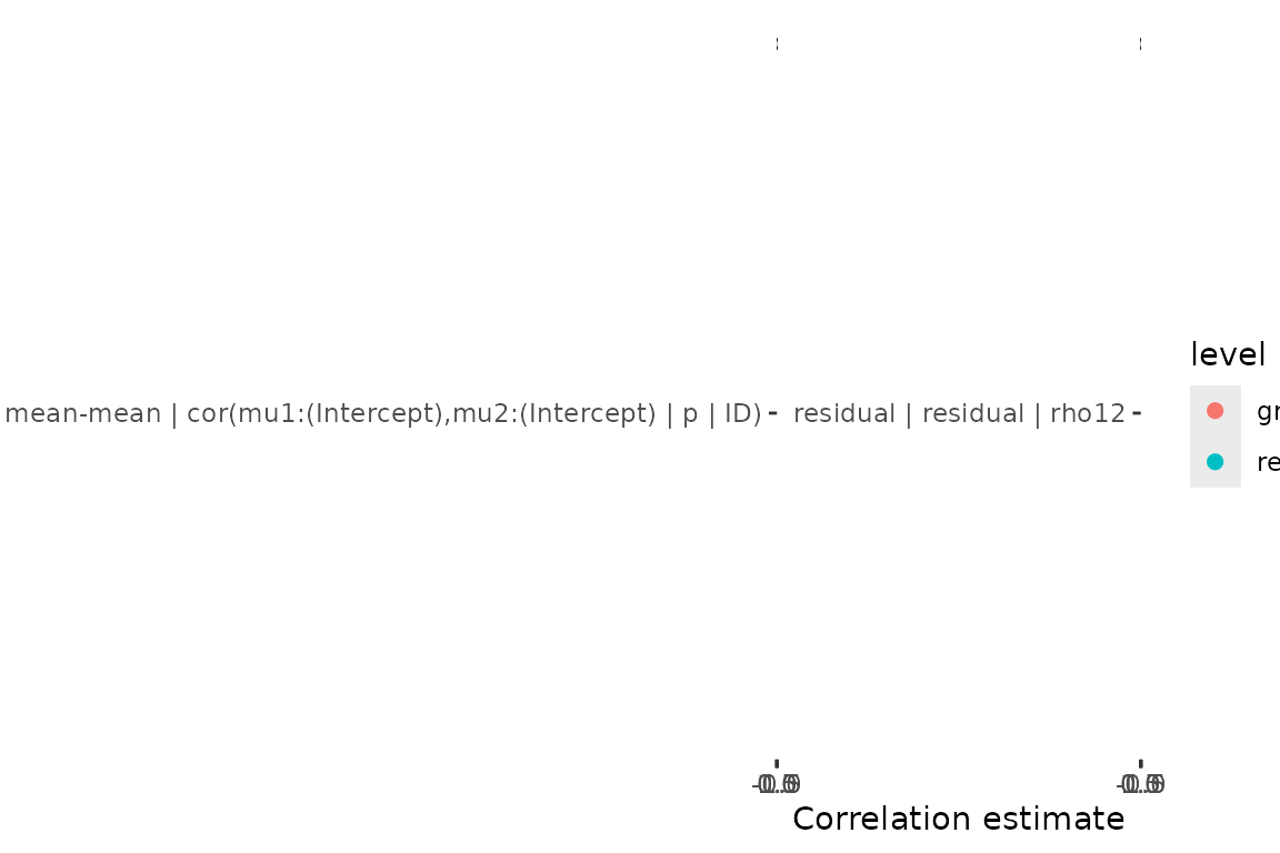
Point plot comparing residual rho12 correlation with the individual-level mean-mean random-intercept correlation, with hollow point estimates and a dotted zero line on a correlation scale from minus one to one.

Point display separating residual rho12 from the individual-level mean-mean random-intercept correlation; the dotted line marks zero correlation. The group row is not shown with an interval because coverage-backed validation remains planned.

The residual row is rho12: within-observation activity-boldness coupling. The group row is the mu1/mu2 random-intercept correlation: among-individual covariation in average activity and average boldness.

summary(fit_group)$covariance gives the same group-level row with the component SDs and covariance on the interpretation scale:

group_covariance <- summary(fit_group)$covariance
report_group_covariance <- group_covariance[
  ,
  c(
    "level", "group", "block", "from_response", "to_response", "class",
    "correlation", "from_sd", "to_sd", "covariance", "from_scale",
    "to_scale", "covariance_conf.status"
  )
]
numeric_columns <- vapply(report_group_covariance, is.numeric, logical(1))
report_group_covariance[numeric_columns] <- lapply(
  report_group_covariance[numeric_columns],
  round,
  3
)
report_group_covariance
#>   level group block from_response to_response     class correlation from_sd
#> 1 group    ID     p      activity    boldness mean-mean       0.475   0.626
#>   to_sd covariance from_scale to_scale covariance_conf.status
#> 1 0.643      0.191   identity identity          not_requested

For this mean-mean block, from_sd is the among-individual SD in average activity and to_sd is the among-individual SD in average boldness. The correlation column is the individual-level activity-boldness correlation, and covariance is correlation * from_sd * to_sd. The identity scale columns tell you these quantities are on the response-location scale, not on a log residual-SD scale.

For this fitted block, check_drm() reports whether group levels are replicated and whether either group-level SD is tiny relative to the matching residual scale. A note there is not a proof that the model is wrong; it tells you to inspect whether the group-level SDs and correlation are supported by the data before treating them as biological conclusions.

Use profile_targets(fit_group) before requesting profile intervals for this block. The SDs are direct random-effect targets, while the modelled corpair() row is a fixed-effect target on the correlation-link scale:

group_targets <- profile_targets(fit_group)
group_cor_dpar <- 'corpair(ID, level = "group", block = "p", from = "mu1", to = "mu2")'
group_target_names <- c(
  "sd:mu:mu1:(1 | p | ID)",
  "sd:mu:mu2:(1 | p | ID)",
  paste0("fixef:", group_cor_dpar, ":(Intercept)")
)
group_targets[
  match(group_target_names, group_targets$parm),
  c("parm", "profile_ready", "profile_note")
]
#>                                                                                     parm
#> 13                                                                sd:mu:mu1:(1 | p | ID)
#> 14                                                                sd:mu:mu2:(1 | p | ID)
#> 9  fixef:corpair(ID, level = "group", block = "p", from = "mu1", to = "mu2"):(Intercept)
#>    profile_ready profile_note
#> 13          TRUE        ready
#> 14          TRUE        ready
#> 9           TRUE        ready

The group-level SD targets are named like sd:mu:mu1:(1 | p | id) and sd:mu:mu2:(1 | p | id). The modelled group-level correlation target begins with fixef:corpair(...). A confint(..., newdata = ...) call can diagnose its response-scale profile geometry, but that callable target is not coverage-backed interval evidence and was not used in the point-only plot. These targets are separate from residual rho12. Returned diagnostic profile rows include profile.boundary and profile.message; a non-"ok" message is a prompt to inspect check_drm(fit) and the profile path.

First slope-slope covariance slice

The first ordinary bivariate random-slope route asks a narrower plasticity-syndrome question: do individuals with steeper response-1 slopes also tend to have steeper response-2 slopes for the same predictor? It is a group-level covariance question, not residual rho12.

For a shared predictor x, the fitted mean layer is:

$\begin{aligned} \mu_{1ij} &= X_{\mu 1}[ij, ]\beta_{\mu 1} + x_{ij}b_{1j},\\ \mu_{2ij} &= X_{\mu 2}[ij, ]\beta_{\mu 2} + x_{ij}b_{2j},\\ \begin{bmatrix} b_{1j}\\ b_{2j} \end{bmatrix} &\sim \operatorname{MVN}(\mathbf{0}, \Sigma_{\mu,x,ID}). \end{aligned}$

The matching first-slice syntax uses slope-only labelled blocks in both location formulas:

drmTMB(
  bf(
    mu1 = y1 ~ x + (0 + x | p | id),
    mu2 = y2 ~ x + (0 + x | p | id),
    sigma1 = ~1,
    sigma2 = ~1,
    rho12 = ~1
  ),
  family = biv_gaussian(),
  data = dat
)

Read this model through sdpars$mu for the two response-specific slope SDs, corpairs(fit, class = "slope-slope") for the group-level slope-slope correlation, summary(fit)$covariance for the covariance table, and profile_targets(fit) for the direct SD and correlation target names. Run check_drm(fit) before interpreting the row; the relevant diagnostic is the bivariate mu random-effect covariance check, plus the ordinary convergence, Hessian, and boundary checks.

This slope-only route deliberately excludes random intercepts from the same labelled bivariate block. If the scientific question needs baseline individual differences and slope differences in the same two-response block, matching q4 and q6 location blocks are now source-tested with syntax such as (1 + x | p | id) or (1 + x + z | p | id) in both location formulas. Treat those routes as fitted extractor/profile-target slices rather than a full tutorial or broad simulation claim. Matching q2 sigma1/sigma2 scale-slope blocks and same-response q2 mu/sigma slope covariance are now fitted as their own routes. The first ordinary q8 all-endpoint block has opt-in smoke/recovery artifact tasks; broader p8/q8 variants and coverage or power claims remain planned.

Boundaries for this covariance layer

The middle p in (1 | p | ID) follows grouped covariance-block syntax for correlated group-level effects. This syntax is distinct from residual rho12. Use rho12(fit) for within-observation residual coupling and corpairs(fit, level = "group") for fitted ordinary group-level covariance rows.

This example teaches only the mu1/mu2 random-intercept covariance row. Other implemented ordinary bivariate random-intercept rows include sigma1/sigma2, one same-response mu/sigma pair, and the all-four mu1/mu2/sigma1/sigma2 block. Read the all-four block as six rows: one mu1-mu2 row, four mean-scale rows (mu1-sigma1, mu1-sigma2, mu2-sigma1, and mu2-sigma2), and one sigma1-sigma2 row.

The first ordinary bivariate slope-slope route is now the matching (0 + x | p | id) block in both mu1 and mu2. The first ordinary q8 all-endpoint block is available as a diagnostic artifact lane, not a tutorial or coverage claim. Broader p8/q8 location-scale slope variants, random effects in rho12, bivariate meta_V() plus random effects, mixed-response families, and ordinary spatial group-level covariance remain future work unless a later status map says otherwise. For phylogenetic covariance, use the structural-dependence tutorial and keep those rows separate from both ordinary group-level covariance and residual rho12.