drmTMB deliberately separates residual scale from
group-level scale. This article pairs each piece of R syntax with the
symbolic model it represents. That pairing is the guardrail: before
adding a feature to the package, the R syntax, equations, TMB
parameters, tests, and documentation should describe the same model.
Read this after you have fit a first model in Distributional regression with drmTMB; this guide settles which scale each formula changes before you pick a family in Choosing response families.
Throughout this article, Normal(a, b) uses variance as
the second argument. Thus Normal(mu_i, sigma_i^2) means a
Gaussian distribution with mean mu_i and standard deviation
sigma_i.
For non-Gaussian families, sigma is still the public
variability-facing scale, but its family-specific meaning changes. For
example, beta and NB2 likelihoods use precision-like internal parameters
and Tweedie uses dispersion phi = sigma^2, while
drmTMB reports sigma so that larger fitted
values mean larger modelled variability. See
vignette("distribution-families") for the conversion table
before comparing sigma with phi,
theta, or other software-specific dispersion
parameters.
Residual standard deviation
Implemented:
Symbolically:
The sigma formula models the residual standard
deviation. If gamma_1 is positive, warmer observations have
a larger residual SD around their fitted mean. The coefficient is on the
log-SD scale, so exp(gamma_1) is the multiplicative change
in residual SD for a one-unit change in temperature.
Mean-model random intercept
Implemented:
drmTMB(
  bf(growth ~ temperature + (1 | population), sigma ~ temperature),
  family = gaussian(),
  data = fish
)
Symbolically:
Here sd_mu_population is the among-population SD in
expected growth. It is a group-level scale parameter for the mean model.
It is not the residual standard deviation sigma_ij.
Residual-scale random intercept
Implemented:
drmTMB(
  bf(
    growth ~ temperature + (1 | population),
    sigma ~ temperature + (1 | population)
  ),
  family = gaussian(),
  data = fish
)
Symbolically:
This asks whether populations differ in their residual variability
after the fixed effects in the sigma formula have been
accounted for. It is group-to-group variation in within-population
variability.
It is not the same as asking whether the among-population SD in mean
growth depends on a predictor. That is the
sd(population) ~ x_group model.
Random-effect scale formula
Implemented for one or more distinct unlabelled Gaussian
mu random intercepts:
drmTMB(
  bf(
    growth ~ temperature + (1 | population),
    sigma ~ temperature,
    sd(population) ~ habitat
  ),
  family = gaussian(),
  data = fish
)
Symbolically:
The right-hand side of sd(population) ~ habitat is
group-level. habitat_j must be constant within each
population after missing rows are removed.
This model asks whether among-population differences in expected
growth are larger in some habitats. That is a different question from
sigma ~ habitat, which asks whether individual observations
are more variable around their fitted mean in some habitats.
A compact copy-run example:
set.seed(1)
n_population <- 24
n_each <- 8
population_info <- data.frame(
  population = factor(seq_len(n_population)),
  habitat = rep(c("closed", "open"), length.out = n_population)
)
fish <- population_info[rep(seq_len(n_population), each = n_each), ]
fish$temperature <- rnorm(nrow(fish))

sd_population <- exp(-0.4 + 0.5 * (population_info$habitat == "open"))
b_population <- rnorm(n_population, sd = sd_population)
sigma <- exp(-0.6 + 0.25 * fish$temperature)
fish$growth <- 1 + 0.7 * fish$temperature +
  b_population[fish$population] +
  rnorm(nrow(fish), sd = sigma)

fit <- drmTMB(
  bf(
    growth ~ temperature + (1 | population),
    sigma ~ temperature,
    sd(population) ~ habitat
  ),
  family = gaussian(),
  data = fish
)

coef(fit, "sd(population)")
head(predict(fit, dpar = "sd(population)"))
The sd(population) coefficients are on the log-SD scale.
A positive habitatopen coefficient means the estimated
among-population SD in expected growth is larger for open-habitat
populations than for the baseline habitat.
One location model, several scale quantities
A model can have one location predictor and several scale quantities. For example, suppose fish growth is measured across populations and sites:
drmTMB(
  bf(
    growth ~ temperature + (1 | population) + (1 | site),
    sigma ~ temperature,
    sd(population) ~ habitat,
    sd(site) ~ site_area
  ),
  family = gaussian(),
  data = fish
)
The matching symbolic model is:
This has three scale quantities:
| Quantity | Formula | Interpretation |
|---|---|---|
sigma_i |
sigma ~ temperature |
residual SD for each observation |
sd_mu_population,j |
sd(population) ~ habitat |
among-population SD in expected growth |
sd_mu_site,k |
sd(site) ~ site_area |
among-site SD in expected growth |
There are no random effects in the residual scale unless the
sigma formula contains a term such as
(1 | population). There is also no correlation between the
population and site random effects in this example; they are separate
grouping factors. Correlated random intercept-slope blocks require a
single grouping factor block such as
(1 + temperature | population).
A copy-run scale audit
This section uses one small ecological example to show what each
scale means in fitted output. Suppose growth is a
growth-rate measurement from several populations. Temperature may change
the expected growth rate and the residual SD around that expectation.
Populations may also differ in their mean growth, and that
among-population SD may be larger in one habitat.
set.seed(42)
n_population <- 32
n_each <- 6

population_info <- data.frame(
  population = factor(seq_len(n_population)),
  habitat = rep(c("forest", "grassland"), length.out = n_population)
)

fish <- population_info[rep(seq_len(n_population), each = n_each), ]
fish$temperature <- rnorm(nrow(fish))
fish$reliability <- ifelse(seq_len(nrow(fish)) %% 3 == 0, 2, 1)

pop_sd <- exp(-0.8 + 0.7 * (population_info$habitat == "grassland"))
b_population <- rnorm(n_population, sd = pop_sd)
fish$sigma_true <- exp(-0.7 + 0.3 * fish$temperature)
fish$growth <- 1.2 + 0.55 * fish$temperature +
  b_population[fish$population] +
  rnorm(nrow(fish), sd = fish$sigma_true)
Residual scale: sigma ~ temperature
The model
is fitted by:
fit_sigma <- drmTMB(
  bf(growth ~ temperature, sigma ~ temperature),
  family = gaussian(),
  data = fish
)

summary(fit_sigma)
#> <summary.drmTMB>
#> estimator: ML
#>                      estimate  std_error
#> mu:(Intercept)     1.19172877 0.06698466
#> mu:temperature     0.46415616 0.06643181
#> sigma:(Intercept) -0.09186998 0.05106557
#> sigma:temperature  0.11531674 0.04798642
#> Distributional, random-effect, scale, and correlation parameters:
#>                         component  dpar         term  estimate   minimum
#> fitted:sigma distributional-scale sigma fitted range 0.9138027 0.6459563
#>               maximum    scale
#> fitted:sigma 1.245707 response
#> logLik: -253.9
#> convergence: 0
round(coef(fit_sigma, "sigma"), 3)
#> (Intercept) temperature
#>      -0.092       0.115
round(range(sigma(fit_sigma)), 3)
#> [1] 0.646 1.246
The sigma:temperature coefficient is on the log-SD
scale. A positive value means residual variation in growth is larger at
warmer temperatures, after the mean temperature effect has been
modelled. The displayed range of sigma(fit) is on the
response scale, so it is the fitted residual SD, not a variance.
Plot the residual scale on its own fitted axis. The raw response
points belong on a growth axis, not on a sigma
axis:
sigma_temperature_grid <- prediction_grid(
  fit_sigma,
  focal = "temperature",
  at = list(
    temperature = seq(
      min(fish$temperature),
      max(fish$temperature),
      length.out = 80
    )
  )
)

sigma_temperature_surface <- predict_parameters(
  fit_sigma,
  newdata = sigma_temperature_grid,
  dpar = "sigma",
  conf.int = TRUE
)

unique(sigma_temperature_surface[, c(
  "dpar",
  "conf.status",
  "interval_source",
  "conf.level"
)])
#>    dpar conf.status interval_source conf.level
#> 1 sigma        wald            wald       0.95

if (requireNamespace("ggplot2", quietly = TRUE)) {
  plot_parameter_surface(
    sigma_temperature_surface,
    x = "temperature",
    dpar = "sigma",
    facet = NULL,
    point = FALSE
  ) +
    ggplot2::labs(
      title = "Residual scale is observation-level",
      subtitle = "Ribbon is a 95% Wald band for fitted sigma",
      x = "Temperature",
      y = "Fitted residual SD (sigma)"
    ) +
    which_scale_theme()
}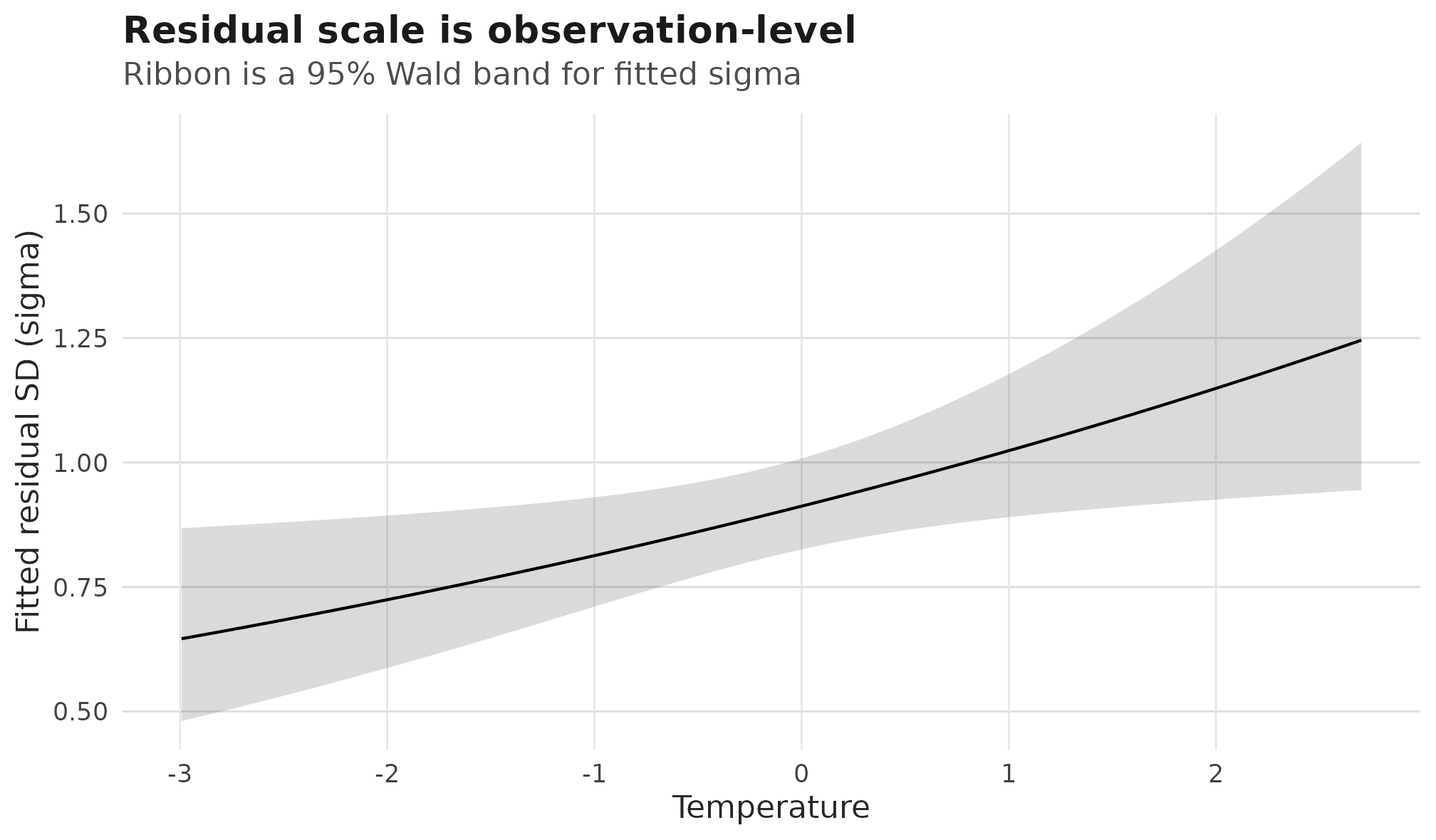
Fitted residual standard deviation over temperature for the
sigma ~ temperature example; the ribbon is a 95% Wald
confidence band from predict_parameters().
Likelihood weights: weights = reliability
Likelihood weights do not define a new biological scale. They multiply the row log-likelihood contribution:
The model syntax stays ordinary:
fit_weighted <- drmTMB(
  bf(growth ~ temperature, sigma ~ 1),
  family = gaussian(),
  data = fish,
  weights = reliability
)

summary(fit_weighted)
#> <summary.drmTMB>
#> estimator: ML
#>                      estimate  std_error
#> mu:(Intercept)     1.18490245 0.05749003
#> mu:temperature     0.47160133 0.05886280
#> sigma:(Intercept) -0.08396322 0.04419416
#> Distributional, random-effect, scale, and correlation parameters:
#>                  component  dpar       term  estimate  std_error    scale
#> sigma distributional-scale sigma (constant) 0.9194651 0.04063499 response
#> logLik: -341.8
#> convergence: 0
head(weights(fit_weighted), 8)
#> [1] 1 1 2 1 1 2 1 1
Here rows with reliability = 2 count twice in the
likelihood. That may be a reasonable model-fitting choice for replicated
or reliability-weighted rows, but it is not the same as telling the
model that an effect size has known sampling variance. Known sampling
variance belongs in meta_V(V = V); deprecated
meta_known_V(V = V) remains a compatibility alias. At
present, dense full known-covariance models reject non-unit likelihood
weights; keep row weighting and known sampling covariance as separate
modelling decisions unless the fitted model explicitly supports their
combination.
Known sampling variance: meta_V(V = V)
For meta-analysis, the known sampling variance is part of the observation model. In a diagonal Gaussian meta-analysis:
The R syntax puts the known variance in the formula, not in
weights:
set.seed(101)
n_effect <- 50
meta <- data.frame(treatment = rep(c(0, 1), each = n_effect / 2))
meta$vi <- runif(n_effect, 0.02, 0.08)

mu_meta <- 0.1 + 0.25 * meta$treatment
sigma_meta <- exp(-1.1 + 0.35 * meta$treatment)
meta$yi <- rnorm(n_effect, mu_meta, sqrt(meta$vi + sigma_meta^2))

fit_meta <- drmTMB(
  bf(yi ~ treatment + meta_V(V = vi), sigma ~ treatment),
  family = gaussian(),
  data = meta
)

summary(fit_meta)
#> <summary.drmTMB>
#> estimator: ML
#>                      estimate  std_error
#> mu:(Intercept)     0.03800893 0.08080623
#> mu:treatment       0.30951079 0.12620218
#> sigma:(Intercept) -1.09445610 0.20331278
#> sigma:treatment    0.26156272 0.26511052
#> Distributional, random-effect, scale, and correlation parameters:
#>                         component  dpar         term  estimate   minimum
#> fitted:sigma distributional-scale sigma fitted range 0.3847555 0.3347216
#>                maximum    scale
#> fitted:sigma 0.4347895 response
#> logLik: -29.79
#> convergence: 0

meta_report <- data.frame(
  treatment = meta$treatment,
  known_sampling_variance = meta$vi,
  extra_heterogeneity_sd = sigma(fit_meta)
)
meta_report$extra_heterogeneity_variance <-
  meta_report$extra_heterogeneity_sd^2
meta_report$total_observation_variance <-
  meta_report$known_sampling_variance +
  meta_report$extra_heterogeneity_variance

meta_summary <- aggregate(
  meta_report[c(
    "extra_heterogeneity_sd",
    "extra_heterogeneity_variance",
    "total_observation_variance"
  )],
  by = list(treatment = meta_report$treatment),
  FUN = mean
)
round(meta_summary, 3)
#>   treatment extra_heterogeneity_sd extra_heterogeneity_variance
#> 1         0                  0.335                        0.112
#> 2         1                  0.435                        0.189
#>   total_observation_variance
#> 1                      0.165
#> 2                      0.236
The vi values are known before the model is fitted. The
fitted sigma describes extra heterogeneity after those
known sampling variances have been included. In meta-analysis notation
this extra heterogeneity is often written as tau, but
drmTMB keeps the name sigma so Gaussian
distributional models use one stable scale vocabulary. If the scientific
summary needs a variance, square the fitted sigma to report
extra heterogeneity variance. If it needs the total observation
variance, add the known sampling variance vi. This is a
reporting conversion, not a separate tau ~ formula.
Random-effect scale: sd(population) ~ habitat
Now the question changes again. The model
asks whether the among-population SD in expected growth differs by habitat:
fit_sd <- drmTMB(
  bf(
    growth ~ temperature + (1 | population),
    sigma ~ temperature,
    sd(population) ~ habitat
  ),
  family = gaussian(),
  data = fish
)

round(coef(fit_sd, "sd(population)"), 3)
#>      (Intercept) habitatgrassland
#>           -0.843            0.860
round(tapply(
  predict(fit_sd, dpar = "sd(population)"),
  population_info$habitat,
  mean
), 3)
#>    forest grassland
#>     0.430     1.017
The habitatgrassland coefficient is on the log-SD scale
for the population random intercept. In this example, grassland
populations have a larger fitted among-population SD in expected growth.
That is not residual variation among individual observations; it is
variation among population-level means.
That group-level SD can be plotted as a fitted model quantity. The current prediction table does not attach a supported interval to this modelled random-effect SD surface, so the figure shows point estimates only:
sd_population_rows <- predict_parameters(
  fit_sd,
  dpar = "sd(population)",
  conf.int = TRUE
)
sd_population_rows$habitat <- population_info$habitat[sd_population_rows$row]

unique(sd_population_rows[, c(
  "dpar",
  "component",
  "conf.status",
  "interval_source"
)])
#>             dpar              component      conf.status interval_source
#> 1 sd(population) random-effect-sd-model newdata_required   not_available

sd_population_display <- aggregate(
  estimate ~ habitat,
  data = sd_population_rows,
  FUN = mean
)

if (requireNamespace("ggplot2", quietly = TRUE)) {
  ggplot2::ggplot(
    sd_population_display,
    ggplot2::aes(x = estimate, y = habitat)
  ) +
    ggplot2::geom_point(size = 3, colour = "#D55E00") +
    ggplot2::labs(
      title = "Group-level scale is not residual sigma",
      subtitle = "Points are fitted sd(population); no supported interval is drawn",
      x = "Fitted among-population SD",
      y = NULL
    ) +
    which_scale_theme()
}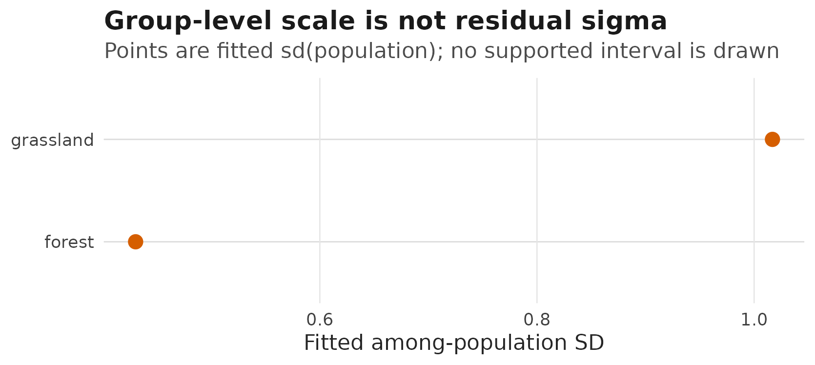
Fitted among-population standard deviations by habitat for the
sd(population) ~ habitat example; points are fitted
random-effect SDs, with no interval drawn because the prediction table
marks this random-effect-SD surface as interval-unavailable.
Residual coscale: rho12 ~ treatment
For two responses, coscale means residual coupling after both response means and residual SDs have been modelled. In the implemented bivariate Gaussian model:
The matching syntax is:
set.seed(12)
behaviour <- data.frame(treatment = rep(c(0, 1), each = 50))
Sigma0 <- matrix(c(0.6^2, 0.2 * 0.6 * 0.5,
                   0.2 * 0.6 * 0.5, 0.5^2), 2, 2)
Sigma1 <- matrix(c(0.6^2, 0.65 * 0.6 * 0.5,
                   0.65 * 0.6 * 0.5, 0.5^2), 2, 2)
Y <- matrix(NA_real_, nrow(behaviour), 2)

for (i in seq_len(nrow(behaviour))) {
  Sigma_i <- if (behaviour$treatment[i] == 0) Sigma0 else Sigma1
  mu_i <- c(1 + 0.2 * behaviour$treatment[i],
            0.5 + 0.1 * behaviour$treatment[i])
  Y[i, ] <- as.numeric(mu_i + t(chol(Sigma_i)) %*% rnorm(2))
}

behaviour$activity <- Y[, 1]
behaviour$boldness <- Y[, 2]

fit_rho12 <- drmTMB(
  bf(
    mu1 = activity ~ treatment,
    mu2 = boldness ~ treatment,
    sigma1 = ~ treatment,
    sigma2 = ~ treatment,
    rho12 = ~ treatment
  ),
  family = c(gaussian(), gaussian()),
  data = behaviour
)

summary(fit_rho12)
#> <summary.drmTMB>
#> estimator: ML
#>                       estimate  std_error
#> mu1:(Intercept)     1.00830416 0.06444478
#> mu1:treatment       0.09996163 0.10841970
#> mu2:(Intercept)     0.46406563 0.06602628
#> mu2:treatment       0.15170720 0.09634348
#> sigma1:(Intercept) -0.78593509 0.10000036
#> sigma1:treatment    0.30225502 0.14142186
#> sigma2:(Intercept) -0.76169095 0.10000004
#> sigma2:treatment    0.06074288 0.14142188
#> rho12:(Intercept)   0.10622747 0.14142197
#> rho12:treatment     0.76355685 0.20000118
#> Distributional, random-effect, scale, and correlation parameters:
#>                          component   dpar         term  estimate   minimum
#> fitted:sigma1 distributional-scale sigma1 fitted range 0.5361019 0.4556934
#> fitted:sigma2 distributional-scale sigma2 fitted range 0.4814955 0.4668763
#> fitted:rho12  residual-correlation  rho12 fitted range 0.4035467 0.1058296
#>                 maximum    scale
#> fitted:sigma1 0.6165104 response
#> fitted:sigma2 0.4961147 response
#> fitted:rho12  0.7012638 response
#> logLik: -130
#> convergence: 0
round(coef(fit_rho12, "rho12"), 3)
#> (Intercept)   treatment
#>       0.106       0.764
round(tapply(rho12(fit_rho12), behaviour$treatment, mean), 3)
#>     0     1
#> 0.106 0.701
The rho12:treatment coefficient is on the
correlation-link scale. The final line shows the same fitted residual
coupling on the response scale. In this simulated example, treatment
changes how tightly activity and boldness remain coupled after their
means and residual SDs have been modelled.
Side-by-side guide
| R syntax | Equation target | Question |
|---|---|---|
sigma ~ x |
log(sigma_i) = X_sigma[i, ] beta_sigma |
Does x change residual SD? |
sigma ~ x + (1 | id) |
log(sigma_i) = X_sigma[i, ] beta_sigma + a_id[i] |
Do groups differ in residual SD? |
sigma ~ x + (0 + w | id) |
log(sigma_i) = X_sigma[i, ] beta_sigma + w_i a_id[i] |
Do groups differ in how w changes residual SD? |
y ~ x + (1 | id) |
mu_i = X_mu[i, ] beta_mu + b_id[i] |
Do groups differ in mean response? |
sd(id) ~ x_group |
log(sd_mu_id,j) = W_id[j, ] alpha_id |
Does x_group change among-group SD in the mean
model? |
weights = w |
logLik = sum_i w_i log f(y_i | theta_i) |
Should row i contribute more or less to the
likelihood? |
meta_V(V = V) |
y ~ MVN(mu, V + Omega_est) |
What sampling covariance is known before fitting? |
y ~ x + (1 + x | id) |
[b_0j, b_1j]' ~ MVN(0, Sigma_id) |
Are group intercepts and slopes correlated? |
rho12 ~ x |
eta_rho12_i = X_rho12[i, ] beta_rho12;
rho12_i = tanh(eta_rho12_i)
|
Does x change residual coupling between two
responses? |
Implementation detail: the C++ likelihood applies a tiny numerical
guard to the tanh() transform so fitted covariance matrices
stay strictly positive definite in floating-point arithmetic. The guard
is not a biological scaling factor. Tutorials and model equations should
be read as the standard Fisher-z-style map from an unconstrained
predictor to a correlation.
Correlations: group-level versus residual
Implemented univariate random-slope correlation:
drmTMB(
  bf(growth ~ temperature + (1 + temperature | population), sigma ~ temperature),
  family = gaussian(),
  data = fish
)
Symbolically:
This rho_re is a group-level random-effect correlation.
It is reported under corpars$mu.
Implemented bivariate residual correlation:
drmTMB(
  bf(
    mu1 = activity ~ treatment,
    mu2 = boldness ~ treatment,
    sigma1 = ~ treatment,
    sigma2 = ~ treatment,
    rho12 = ~ treatment
  ),
  family = c(gaussian(), gaussian()),
  data = behaviour
)
Symbolically:
Here rho12_i is residual response-response correlation
within an observation after the response-specific means and residual SDs
have been modelled. If the correlation is among random intercepts or
random slopes, it is a group-level covariance parameter. If the
correlation is between the two residual responses in one row, it is
rho12. Extract fitted response-scale residual correlations
with rho12(fit). Use corpairs(fit) when you
want a table that keeps residual rho12 separate from
ordinary group-level random-effect correlations, including the
implemented bivariate mu1/mu2,
sigma1/sigma2, and same-response
mu/sigma random-intercept correlations.
Family A versus Family B
Two model families can both sound like “scale random effects”, but they are different likelihoods.
Family A puts random effects inside distributional formulas. For
example, sigma ~ z + (1 | id) adds a group-level
residual-scale deviation to log(sigma_ij). Matching labels
such as (1 | p | id) across mu and
sigma, or across mu1, mu2,
sigma1, and sigma2, define latent covariance
blocks. Read those correlations with corpairs().
Family B models the SD of a location random effect directly. For
example, sd(id) ~ habitat changes the among-id
SD in the mu random intercept. The phylogenetic direct-SD
analogue is spelled
sd(species, level = "phylogenetic") ~ z_species, which is
the current generic syntax. The legacy
sd_phylo(species) ~ z_species spelling is a soft-deprecated
alias (as of 0.3.0): it still parses and fits identically, but emits a
one-time deprecation warning per session and should not be used in new
formulas.
Do not mix the two families for the same latent layer. For example, a
q=4 Family A block with matching labelled phylo() terms in
mu1, mu2, sigma1, and
sigma2 already estimates one constant latent covariance
block. Adding sd1(species, level = "phylogenetic") ~ z or
sd2(species, level = "phylogenetic") ~ z to that same q=4
block would ask for a predictor-dependent direct-SD model at the same
time, so drmTMB() rejects that combination before
fitting.
| Question | Use | Do not read it as |
|---|---|---|
| Do groups differ in residual SD? | sigma ~ ... + (1 | group) |
a model for among-group mean differences |
| Does a group-level predictor change among-group mean SD? | sd(group) ~ x_group |
residual sigma regression |
| Do two latent group effects move together? | matching labelled random effects plus corpairs()
|
residual rho12
|
| Does a species-level predictor change phylogenetic location SD? | sd(species, level = "phylogenetic") ~ z_species |
a q=4 location-scale covariance block |
Current boundary
Current implemented Gaussian syntax covers:
-
sigma ~ xfor residual SD fixed effects; -
y ~ x + (1 | id)formurandom intercepts; -
y ~ x + (0 + x | id)for independent numericmurandom slopes; -
y ~ x + (1 + x | id)and(1 + x | p | id)for one-slope correlatedmublocks; -
y ~ x1 + x2 + x3 + (1 + x1 + x2 + x3 | id)for ordinary q > 2 numeric multi-slopemublocks, where random-slope SDs are direct targets and block correlations are derived-unavailable for direct profile intervals; -
sigma ~ x + (1 | id)for residual-scale random intercepts; -
sigma ~ x + (0 + w | id)andsigma ~ x + (0 + w_id | id) + (0 + w_site | site)for independent residual-scale random slopes, including separate grouping factors; -
sigma ~ x + (1 + w | id)and unlabelled multi-slope variants for fitted within-block residual-scale correlations; -
sd(id) ~ x_groupand multiple distinctsd(group) ~ x_groupformulas for standard deviations of unlabelled Gaussianmurandom intercepts; - bivariate fixed-effect
rho12 ~ xwithfamily = c(gaussian(), gaussian()); - matching labelled
(1 | p | id)random intercepts in bivariatemu1andmu2; - matching labelled
(1 | p | id)random intercepts in bivariatesigma1andsigma2; - one same-response bivariate
mu/sigmarandom-intercept covariance pair, such as matching(1 | p | id)terms inmu1andsigma1; - matching intercept-only
phylo(1 | species, tree = tree)terms in bivariatemu1andmu2, with residualrho12kept as the within-observation residual correlation.
Current planned but not implemented syntax includes:
- slope-specific and labelled-block random-effect scale models;
- labelled residual-scale slope blocks in
sigmaand cross-formula labelledmu/sigmarandom-slope covariance (unlabelled ordinary correlated intercept-slope and multi-slopesigmablocks are fitted); - residual-scale bivariate random slopes and full cross-parameter covariance blocks spanning more than one pair;
- cross-formula covariance sharing from repeated slope labels outside
the matching source-tested bivariate
mu1/mu2q4/q6 location routes; - multiple phylogenetic slopes, phylogenetic slope correlations,
standalone or partial phylogenetic scale terms, predictor-dependent q=4
phylogenetic location-scale correlations, structured
rho12effects, mesh/SPDE spatial fields, spatial slope correlations, and non-Gaussian spatial structured effects outside the exact ordinary Poisson/NB2 q1 spatialmuintercept-plus-one-slope, recovery-grade NB2 q1 spatialsigma, Student-t spatialmu, Poisson spatialzi, fixed-ziPoisson spatialmu, and fixed-ziNB2 spatialmugates.
With the scale vocabulary settled, move on to Choosing response families to pick a family, then to a matching interpretation tutorial such as When variance carries signal, Part 1.