After fitting a distributional model, the next question is not only “what are the coefficients?” A useful workflow checks the fit, extracts the fitted distributional parameters, predicts to meaningful covariate values, examines residuals, and simulates from the fitted model.
This article uses a small growth example, but the same workflow
applies to other Gaussian location-scale models in drmTMB.
Read it after the getting-started fit in Distributional regression with drmTMB and the
model-status map in What can I fit today?:
this page is where estimates become checked tables, predictions,
intervals, residuals, and simulation checks.
Fit the model
Suppose growth is measured along a temperature gradient in two habitat types. The model asks whether temperature and habitat change expected growth, and whether temperature also changes residual variability.
Symbolically:
Matching R syntax:
library(drmTMB)
#>
#> Attaching package: 'drmTMB'
#> The following object is masked from 'package:base':
#>
#>     beta

set.seed(12)
n <- 120
fish <- data.frame(
  temperature = runif(n, -1.5, 1.5),
  habitat = factor(sample(c("reef", "kelp"), n, replace = TRUE))
)
eta_mu <- 1 + 0.7 * fish$temperature + 0.35 * (fish$habitat == "kelp")
eta_sigma <- -0.5 + 0.25 * fish$temperature
fish$growth <- rnorm(n, mean = eta_mu, sd = exp(eta_sigma))

fit <- drmTMB(
  bf(growth ~ temperature + habitat, sigma ~ temperature),
  family = gaussian(),
  data = fish
)
Here growth ~ temperature + habitat defines the location
model, and sigma ~ temperature defines the residual
standard deviation model on the log scale.
Check before interpreting
Run check_drm() before interpreting estimates:
check_drm(fit)
#> <drm_check: 12 checks>
#> ok: 12; notes: 0; warnings: 0; errors: 0
#>                      check status
#>      optimizer_convergence     ok
#>           optimizer_budget     ok
#>           finite_objective     ok
#>      logsigma_clamp_active     ok
#>             fixed_gradient     ok
#>            sdreport_status     ok
#>  hessian_positive_definite     ok
#>     standard_errors_finite     ok
#>   standard_errors_inflated     ok
#>               dropped_rows     ok
#>             positive_scale     ok
#>   fixed_effect_design_size     ok
#>                                                                                   value
#>                                                                                       0
#>                                                 iterations=19; function=31; gradient=19
#>                                                                                   110.6
#>                                                                                    <NA>
#>                                                  max=0.0002814; component=beta_sigma[2]
#>                                                                                      ok
#>                                                                                    TRUE
#>                                                                  range=[0.06459,0.1109]
#>                                          n_inflated=0; max_se=0.1109; median_se=0.08325
#>                                                                     nobs=120; dropped=0
#>                                                                              min=0.4388
#>  total_mb=0.02132; max_cols=3; largest=mu; largest_class=matrix; largest_density=0.8639
#>                                                                              message
#>                                                        nlminb convergence code is 0.
#>  Optimizer evaluation counts recorded; no eval.max or iter.max control was supplied.
#>                                             Objective and log-likelihood are finite.
#>                                   The log(sigma) clamp is not active at the optimum.
#>     Maximum absolute fixed gradient is <= 0.001; largest component is beta_sigma[2].
#>                                              TMB::sdreport() completed successfully.
#>                                        sdreport reports a positive-definite Hessian.
#>                                         All fixed-effect standard errors are finite.
#>                   No fixed-effect standard error is inflated relative to the others.
#>                   No rows were dropped by model-frame or known-covariance filtering.
#>                                     All fitted scale values are finite and positive.
#>                          Dense fixed-effect design matrices are modest for this fit.
A clean diagnostic table does not prove that the model is
scientifically correct, but it catches common problems early: optimizer
convergence, gradients, optimizer evaluation counts, finite objective
values, Hessian status, dropped rows, finite fixed-effect standard
errors, positive scale values, residual rho12 values near
the boundary, Student-t nu values near the boundary or
close to Gaussian behaviour, known sampling covariance summaries,
random-effect standard deviations near zero, and random-effect design
issues when random effects are present.
If check_drm() flags optimizer_convergence
or fixed_gradient, read Improving convergence for the full
diagnostic table before trusting any estimate from that fit.
check_drm() only checks that the optimizer behaved; it
does not ask whether the fitted distribution itself fits the data. For
that question, read Distributional outputs
and adequacy for worm plots, QQ plots, and centile checks once the
optimizer diagnostics are clean.
Read the ordinary summary first
The ordinary R habit is still the right first habit in
drmTMB:
summary(fit)
#> <summary.drmTMB>
#> estimator: ML
#>                     estimate  std_error
#> mu:(Intercept)     1.3217191 0.08692866
#> mu:temperature     0.6576081 0.06883060
#> mu:habitatreef    -0.3776491 0.11093864
#> sigma:(Intercept) -0.4914488 0.06458586
#> sigma:temperature  0.2251861 0.08324785
#> Distributional, random-effect, scale, and correlation parameters:
#>                         component  dpar         term  estimate   minimum
#> fitted:sigma distributional-scale sigma fitted range 0.6188039 0.4388472
#>                maximum    scale
#> fitted:sigma 0.8465434 response
#> logLik: -110.6
#> convergence: 0
summary() puts the fixed-effect estimates,
response-scale scale, shape, random-effect SD, correlation summaries,
fitted covariance summaries, derived variance ratios, log likelihood,
and convergence code in one place when those quantities are present. The
fixed-effect table includes standard errors when
TMB::sdreport() was computed successfully.
Read the printed summary as a map, then use a more specific extractor only when you need more detail:
| Summary component | What it reports | Use it for |
|---|---|---|
coefficients |
Fixed-effect coefficients for each distributional parameter, usually on the model’s link scale. | Direction, sign, and approximate uncertainty of terms in
mu, sigma, rho12, shape, or
zero-inflation formulas. |
parameters |
Direct response-scale parameters, fitted parameter ranges, random-effect SDs, and fitted correlations. | Constant sigma, residual rho12,
sd:mu:(1 | group), and quick response-scale uncertainty
when std_error is available. |
covariance |
Fitted random-effect covariance and correlation rows for supported covariance blocks. | Latent correlation layers such as group-level, phylogenetic, or structured-effect covariance summaries. |
derived |
Simple variance-ratio summaries whose ingredients are unambiguous. | Repeatability or phylogenetic signal point estimates, including the random-effect and residual variances used in the ratio. |
confint |
Confidence-interval rows only when
conf.int = TRUE. |
Checking which requested fixed-effect or profile-likelihood intervals were actually computed. |
The printed summary is meant to answer “what did this fitted model
estimate?” For workflows that need the full object behind a row, use
fixef(), sigma(), rho12(),
ranef(), corpairs(), or
profile_targets() after reading the summary.
The rest of this article turns from ordinary fixed-effect post-fit
checks to models with (1 | site) random intercepts,
sd(site) ~ reef_cover random-effect scale formulas, and
emmeans marginal means. That is random-effects-stage
material: if you have not yet fit a model with a grouping factor, you
can skip ahead to a later worked tutorial and come back to this section
once you have.
For models with random effects, summary() is also the
first place to look for variance components. This compact example adds a
site random intercept to the location model:
set.seed(13)
n_site <- 18
n_per_site <- 6
site <- factor(rep(seq_len(n_site), each = n_per_site))
site_effect <- rnorm(n_site, sd = 0.45)

fish_site <- data.frame(
  site = site,
  temperature = runif(n_site * n_per_site, -1.5, 1.5),
  habitat = factor(
    sample(c("reef", "kelp"), n_site * n_per_site, replace = TRUE)
  )
)

site_mu <- site_effect[as.integer(fish_site$site)]
fish_site$growth <- rnorm(
  nrow(fish_site),
  mean = 1 + 0.7 * fish_site$temperature +
    0.35 * (fish_site$habitat == "kelp") + site_mu,
  sd = 0.35
)

fit_site <- drmTMB(
  bf(growth ~ temperature + habitat + (1 | site), sigma ~ 1),
  family = gaussian(),
  data = fish_site
)

summary(fit_site)
#> <summary.drmTMB>
#> estimator: ML
#>                     estimate  std_error
#> mu:(Intercept)     1.3588788 0.10385484
#> mu:temperature     0.6814229 0.04764308
#> mu:habitatreef    -0.2416812 0.07768774
#> sigma:(Intercept) -0.9603029 0.07455733
#> Distributional, random-effect, scale, and correlation parameters:
#>                             component  dpar       term  estimate  std_error
#> sigma            distributional-scale sigma (constant) 0.3827769 0.02853883
#> sd:mu:(1 | site)     random-effect-sd    mu (1 | site) 0.3721619 0.07323934
#>                     scale
#> sigma            response
#> sd:mu:(1 | site) response
#> Derived summaries:
#>                                  quantity level group       term  estimate
#> derived:repeatability(site) repeatability group  site (1 | site) 0.4859419
#>                             random_effect_variance residual_variance
#> derived:repeatability(site)              0.1385045         0.1465182
#> logLik: -66.61
#> convergence: 0
In that output, the sd:mu:(1 | site) row is the fitted
random-intercept standard deviation on the response scale. Squaring it
gives the corresponding random-effect variance component. When the
ingredients are unambiguous, the derived component also
reports repeatability and shows both the random-effect variance and the
residual variance used in that ratio.
Once you have more than one candidate model fitted to the same data — for example this random-intercept model against a simpler fixed-effect version — read Model selection with AIC and BIC to choose between them rather than reporting whichever one was fit last.
When TMB::sdreport() succeeds, direct response-scale
parameter rows such as constant sigma and
sd:mu:(1 | site) also include delta-method standard errors.
confint() uses those same optimized-parameter covariances
for its fast default Wald intervals. SD intervals are formed on the
fitted log-SD scale and exponentiated; correlation intervals are formed
on the fitted guarded atanh scale and transformed back with the model’s
correlation transform. Treat these as quick local approximations, then
reserve profile or bootstrap work for the SD or correlation rows that
need likelihood-shape or refit-based uncertainty. drmTMB is
a frequentist package, so these are confidence intervals, not Bayesian
credible intervals:
profile_targets(fit_site)
#>                          parm         target_class  dpar        term
#> 1        fixef:mu:(Intercept)         fixed-effect    mu (Intercept)
#> 2        fixef:mu:temperature         fixed-effect    mu temperature
#> 3        fixef:mu:habitatreef         fixed-effect    mu habitatreef
#> 4     fixef:sigma:(Intercept)         fixed-effect sigma (Intercept)
#> 5                       sigma distributional-scale sigma  (constant)
#> 6            sd:mu:(1 | site)     random-effect-sd    mu  (1 | site)
#> 7 derived:repeatability(site)      derived-summary    mu  (1 | site)
#>   tmb_parameter index   estimate link_estimate    scale   transformation
#> 1       beta_mu     1  1.3588788     1.3588788     link linear_predictor
#> 2       beta_mu     2  0.6814229     0.6814229     link linear_predictor
#> 3       beta_mu     3 -0.2416812    -0.2416812     link linear_predictor
#> 4    beta_sigma     1 -0.9603029    -0.9603029     link linear_predictor
#> 5    beta_sigma     1  0.3827769    -0.9603029 response              exp
#> 6     log_sd_mu     1  0.3721619    -0.9884264 response              exp
#> 7          <NA>    NA  0.4859419            NA response   variance_ratio
#>   target_type profile_ready   profile_note
#> 1      direct          TRUE          ready
#> 2      direct          TRUE          ready
#> 3      direct          TRUE          ready
#> 4      direct          TRUE          ready
#> 5      direct          TRUE          ready
#> 6      direct          TRUE          ready
#> 7     derived         FALSE derived_target
The fastest fitted-model interval check is the default Wald route:
confint(fit_site)
#>                      parm level      lower       upper    scale
#> 1    fixef:mu:(Intercept)  0.95  1.1553271  1.56243054     link
#> 2    fixef:mu:temperature  0.95  0.5880442  0.77480166     link
#> 3    fixef:mu:habitatreef  0.95 -0.3939464 -0.08941602     link
#> 4 fixef:sigma:(Intercept)  0.95 -1.1064326 -0.81417319     link
#> 5                   sigma  0.95  0.3307367  0.44300546 response
#> 6        sd:mu:(1 | site)  0.95  0.2530581  0.54732274 response
#>     transformation tmb_parameter index method profile.engine conf.status
#> 1 linear_predictor       beta_mu     1   wald           <NA>        wald
#> 2 linear_predictor       beta_mu     2   wald           <NA>        wald
#> 3 linear_predictor       beta_mu     3   wald           <NA>        wald
#> 4 linear_predictor    beta_sigma     1   wald           <NA>        wald
#> 5              exp    beta_sigma     1   wald           <NA>        wald
#> 6              exp     log_sd_mu     1   wald           <NA>        wald
#>   profile.boundary profile.message
#> 1               NA            <NA>
#> 2               NA            <NA>
#> 3               NA            <NA>
#> 4               NA            <NA>
#> 5               NA            <NA>
#> 6               NA            <NA>
For a long mixed or phylogenetic model, narrow the table before doing anything expensive:
confint(fit_site, parm = "variance_components")
#>               parm level     lower     upper    scale transformation
#> 1            sigma  0.95 0.3307367 0.4430055 response            exp
#> 2 sd:mu:(1 | site)  0.95 0.2530581 0.5473227 response            exp
#>   tmb_parameter index method profile.engine conf.status profile.boundary
#> 1    beta_sigma     1   wald           <NA>        wald               NA
#> 2     log_sd_mu     1   wald           <NA>        wald               NA
#>   profile.message
#> 1            <NA>
#> 2            <NA>
When the interval table is not enough, inspect the likelihood shape
directly. The curve below profiles the constant residual
sigma target from the same site model. The y-axis is
likelihood-ratio distance; the solid vertical line is the fitted
sigma, the dotted horizontal line is the 95% profile
cutoff, and the dashed vertical lines are the profile confidence
endpoints:
if (requireNamespace("ggplot2", quietly = TRUE)) {
  site_sigma_profile <- stats::profile(
    fit_site,
    parm = "sigma",
    level = 0.95,
    trace = FALSE,
    profile_precision = "fast"
  )

  plot(site_sigma_profile) +
    workflow_theme() +
    ggplot2::labs(
      title = "Profile shape for residual sigma",
      subtitle = "Fast full-profile pass for one direct target",
      x = "Residual sigma (response scale)"
    )
}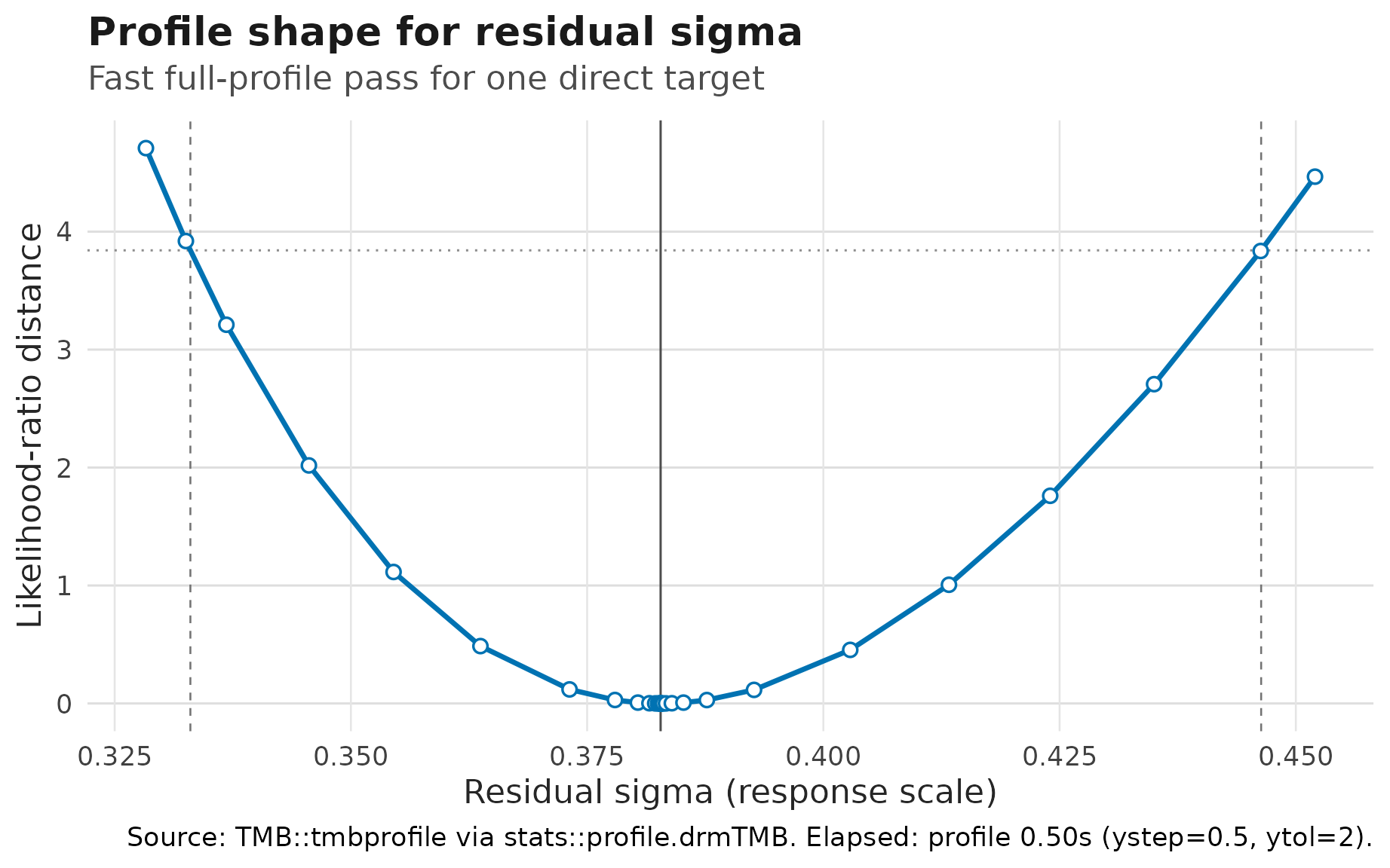
Profile-likelihood curve for constant residual sigma in the
site random-intercept model. The curve is likelihood-ratio distance on
the public positive sigma scale; dashed lines mark 95%
profile confidence endpoints.
The variance-component shortcut returns constant scale targets and
direct random-effect SD targets. The companion shortcuts
"fixed_effects", "random_effects", and
"correlations" keep large interval tables readable. For a
diagnostic likelihood profile of a specific SD or correlation row, copy
the exact target name from profile_targets() and profile
only that target. Profile availability alone is not coverage-backed
interval validation; confirm the exact row in the capability guide
before reporting it. profile_precision = "fast" supplies
coarser TMB::tmbprofile() controls
(ystep = 0.5, ytol = 2) unless you override
them in ...; it is useful as a first pass for long
phylogenetic or spatial SD profiles:
summary(
  fit_site,
  conf.int = TRUE,
  method = "profile",
  ci_parm = "sd:mu:(1 | site)",
  profile_precision = "fast"
)
The same target can be requested directly:
confint(
  fit_site,
  parm = "sd:mu:(1 | site)",
  method = "profile",
  profile_precision = "fast"
)
When refit-based uncertainty is the point of the analysis, use the
bounded bootstrap route in confint() for selected direct
targets. Start with a small pilot to estimate runtime, then increase
R for the final analysis:
confint(
  fit_site,
  parm = "variance_components",
  method = "bootstrap",
  R = 99,
  seed = 20260521
)
Bootstrap rows record successful and failed refits in
bootstrap.n and bootstrap.failed. The returned
interval table also carries a "bootstrap.diagnostics"
attribute with one row per refit and target, so failed or missing draws
can be inspected without changing the printed interval table. On
Unix-like systems, parallel = "multicore" and
workers = ... can run refits in parallel;
drmTMB caps bootstrap workers at 10 to avoid accidental
oversubscription.
Each distributional parameter has its own coefficient vector:
coef(fit, "mu")
#> (Intercept) temperature habitatreef
#>   1.3217191   0.6576081  -0.3776491
coef(fit, "sigma")
#> (Intercept) temperature
#>  -0.4914488   0.2251861
The sigma coefficients are on the log-standard-deviation
scale. A positive temperature coefficient in sigma means
that residual variability increases with temperature. Exponentiating the
coefficient gives a multiplicative change in residual standard deviation
for a one-unit temperature increase.
Use the scale of the fitted parameter when deciding what to report:
| Output | Fitted scale | Report when the question is… |
|---|---|---|
coef(fit, "mu") |
response units | expected growth, treatment effects, or mean trait differences |
coef(fit, "sigma") |
log residual SD | multiplicative residual-SD or residual-variance contrasts |
sigma(fit) |
residual SD | fitted predictability or extra heterogeneity on the response scale |
rho12(fit) |
residual correlation | residual coupling between two responses after means and residual SDs are modelled |
corpairs(fit) |
fitted correlation rows | group-level, phylogenetic, or residual correlation layers, depending
on level
|
profile_targets(fit) |
interval target inventory | whether a fitted SD or correlation target can receive a profile interval |
For confidence intervals, keep the fast default summary separate from the expensive profile or bootstrap step. Wald 95% confidence intervals are available for fixed effects and direct response-scale parameter rows:
summary(fit, conf.int = TRUE)
#> <summary.drmTMB>
#> estimator: ML
#> confidence intervals: wald, level = 0.95
#>                     estimate  std_error    conf.low  conf.high conf.level
#> mu:(Intercept)     1.3217191 0.08692866  1.15134209  1.4920962       0.95
#> mu:temperature     0.6576081 0.06883060  0.52270265  0.7925136       0.95
#> mu:habitatreef    -0.3776491 0.11093864 -0.59508488 -0.1602134       0.95
#> sigma:(Intercept) -0.4914488 0.06458586 -0.61803474 -0.3648628       0.95
#> sigma:temperature  0.2251861 0.08324785  0.06202331  0.3883489       0.95
#>                   conf.method conf.status profile.boundary profile.message
#> mu:(Intercept)           wald        wald               NA            <NA>
#> mu:temperature           wald        wald               NA            <NA>
#> mu:habitatreef           wald        wald               NA            <NA>
#> sigma:(Intercept)        wald        wald               NA            <NA>
#> sigma:temperature        wald        wald               NA            <NA>
#> Distributional, random-effect, scale, and correlation parameters:
#>                         component  dpar         term  estimate   minimum
#> fitted:sigma distributional-scale sigma fitted range 0.6188039 0.4388472
#>                maximum    scale      conf.status
#> fitted:sigma 0.8465434 response wald_unavailable
#> logLik: -110.6
#> convergence: 0
Fixed effects include distributional-parameter coefficients such as
sigma, Student-t nu, zero-inflation, hurdle,
and residual rho12 formula terms. Those Wald intervals are
on the fitted link scale. For example, a Student-t
fixef:nu:x row is an interval for the
log(nu - 2) coefficient, not a response-scale
degrees-of-freedom interval at a particular covariate value.
Profile-likelihood 95% confidence intervals are available for
selected direct targets such as constant sigma,
random-effect SDs, random-effect correlations, and constant residual
rho12. Fixed effects keep Wald confidence intervals in the
same profile summary unless fixed-effect profile targets are selected.
For example, fit_site has sigma ~ 1, so its
residual standard deviation is a direct fitted-object target:
summary(fit_site, conf.int = TRUE, method = "profile", ci_parm = "sigma")For the first model in this article, sigma depends on
temperature. There is no single response-scale
sigma target until you name the covariate row you want to
profile:
sigma_grid <- data.frame(
  temperature = c(-1, 1),
  habitat = factor("reef", levels = levels(fish$habitat))
)
row.names(sigma_grid) <- c("cool_reef", "warm_reef")

confint(fit, parm = "sigma", method = "profile", newdata = sigma_grid)
The same row-specific rule applies to bivariate Gaussian scale and
residual correlation models. In a two-response fit with
sigma1 ~ z1, sigma2 ~ z2, and
rho12 ~ w, profile the biologically meaningful rows
directly. A predictor-dependent parameter has no single scalar target,
which is why newdata is required: without it the summary
reports conf.status = "newdata_required" rather than an
interval. These row-specific intervals are computed but not
coverage-certified. The constant rho12 ~ 1 profile interval
is likewise interval-feasible rather than coverage-certified: the
current ledger records no committed bivariate fixed-effect CI-coverage
simulation for either form.
biv_grid <- data.frame(
  x = 0,
  z1 = c(-1, 1),
  z2 = c(1, -1),
  w = c(-0.5, 0.5)
)
row.names(biv_grid) <- c("cool_low_coupling", "warm_high_coupling")

confint(fit_biv, parm = "sigma1", method = "profile", newdata = biv_grid)
confint(fit_biv, parm = "sigma2", method = "profile", newdata = biv_grid)
confint(fit_biv, parm = "rho12", method = "profile", newdata = biv_grid)
For diagnostic profiles of random-effect SDs and correlations, copy
the exact target name from profile_targets(). Random-slope
terms keep the coefficient suffix in the target name, and residual
rho12 remains separate from group-level or phylogenetic
correlation rows. A callable target demonstrates mechanics, not
coverage-backed interval validation for that model cell:
profile_targets(fit_slope)

summary(
  fit_slope,
  conf.int = TRUE,
  method = "profile",
  ci_parm = "sd:mu:(1 + temperature | p | site):temperature"
)
summary(
  fit_slope,
  conf.int = TRUE,
  method = "profile",
  ci_parm = "cor:mu:cor((Intercept),temperature | p | site)"
)
summary(
  fit_biv_group,
  conf.int = TRUE,
  method = "profile",
  ci_parm = "cor:mu:cor(mu1:(Intercept),mu2:(Intercept) | p | id)"
)
Use these calls to inspect profile geometry. Successful profile rows
include profile.boundary and profile.message;
values other than "ok" flag boundary or
near-correlation-limit behaviour. Before reporting a variance-component,
SD, or correlation interval, also confirm that the exact row is
interval-validated in the capability guide; profile availability alone
is not that evidence.
For correlations, the fast Wald route uses the model’s fitted
correlation-link scale, which is a guarded Fisher-z/atanh transform for
current correlation parameters. This differs from a sample-correlation
Fisher-z interval with an effective sample size: drmTMB is
using the TMB covariance of the fitted correlation parameter, not a
separate n_eff heuristic.
Use profile_targets(fit) before asking for a profile
interval. A row is profile-ready only when it maps to a direct TMB
target and the fitted object kept its TMB object. Interval-aware output
uses conf.status to explain rows without intervals:
newdata_required means profile a supplied row with
confint(..., newdata = ...), while
derived_interval_unavailable means the point estimate
combines several quantities and needs a later derived-profile
method.
Read conf.status as an action column:
conf.status |
What it means | What to do next |
|---|---|---|
wald |
A Wald interval was returned for a fixed-effect or direct parameter row. | Use it for routine summaries and as the fastest screen for large models, while remembering it is asymptotic. |
profile |
A profile-likelihood interval was returned. | Inspect profile.boundary and
profile.message before treating the interval as
stable. |
bootstrap |
A simulate/refit percentile interval was returned by
confint(). |
Check bootstrap.n, bootstrap.failed, and
attr(ci, "bootstrap.diagnostics"); increase R
only after a small runtime pilot works. |
profile_ready |
The row is a direct profile target, but the current summary call did not request it. | Use the row’s parm value in
confint(..., method = "profile") or in
summary(..., method = "profile", ci_parm = ...). |
newdata_required |
The fitted surface needs a concrete row before it can be profiled. | Build a biologically meaningful newdata row and call
confint(..., newdata = ...). |
derived_interval_unavailable |
The point estimate combines multiple fitted quantities and has no validated interval method yet. | Report the point estimate as exploratory, or simplify to a direct target if interval support is essential. |
wald_unavailable |
Wald uncertainty is not available for this row, or
sdreport() was skipped or failed. |
Use a profile-ready target when one exists; otherwise report the missing interval explicitly. |
bootstrap_unavailable |
Fewer than two bootstrap refits produced a finite estimate for the requested target. | Treat the interval as unavailable; inspect model convergence, refit
controls, and attr(ci, "bootstrap.diagnostics") before
increasing R. |
target_unavailable or
profile_unavailable
|
The row is descriptive or has no current direct interval target. | Treat the interval as unsupported and check
profile_targets(fit) before trying another route. |
not_requested |
The table is reporting a point estimate without an interval request. | Refit is not needed; request intervals only for the rows you plan to interpret. |
Bootstrap intervals are public only through confint()
for selected direct targets.
summary(fit, conf.int = TRUE, method = "bootstrap") and
corpairs(fit, conf.int = TRUE, method = "bootstrap") still
stop before interval work begins, and derived q4 covariance rows,
repeatability, and phylogenetic signal still need separate interval
designs. For long applied models, the practical default is therefore:
Wald for routine reporting, targeted
profile_precision = "fast" profile checks for important SD
or correlation rows, and bootstrap only when refit-based uncertainty is
worth the runtime.
Predict distributional parameters
predict() returns one distributional parameter at a
time. For fitted rows, fitted(fit) and
predict(fit, dpar = "mu") return the same location values
for this fixed-effect model:
head(fitted(fit))
#> [1] 0.4721438 1.5709847 2.1949341 0.8667501 0.2917519 0.4021770
head(predict(fit, dpar = "mu"))
#> [1] 0.4721438 1.5709847 2.1949341 0.8667501 0.2917519 0.4021770
head(sigma(fit))
#> [1] 0.4573206 0.7582265 0.8249504 0.5234861 0.4892785 0.4464939
For new covariate values, supply newdata. These are
fixed-effect, population-level predictions. You can write the grid
directly:
new_fish <- data.frame(
  temperature = c(-1, 0, 1),
  habitat = factor("reef", levels = levels(fish$habitat))
)

predict(fit, newdata = new_fish, dpar = "mu")
#> [1] 0.2864619 0.9440700 1.6016782
predict(fit, newdata = new_fish, dpar = "sigma")
#> [1] 0.4883930 0.6117395 0.7662378
predict(fit, newdata = new_fish, dpar = "sigma", type = "link")
#> [1] -0.7166349 -0.4914488 -0.2662627
Or build an explicit prediction grid. This keeps the focal term, conditioned nuisance predictors, and grid rule attached to the data:
temperature_grid <- prediction_grid(
  fit,
  focal = "temperature",
  at = list(temperature = c(-1, 0, 1)),
  condition = list(habitat = "reef")
)

attr(temperature_grid, "prediction_grid")
#> $focal_terms
#> [1] "temperature"
#>
#> $conditioned_terms
#> [1] "habitat"
#>
#> $margin
#> [1] "mean_reference"
#>
#> $weights
#> [1] "equal"
#>
#> $grid_source
#> [1] "mean_reference_prediction_grid"
#>
#> $reference_terms
#> character(0)
#>
#> $predictor_terms
#> [1] "temperature" "habitat"
#>
#> $n_source_rows
#> [1] 120
#>
#> $n_grid_rows
#> [1] 3
Use predict_parameters() when the interpretation task
needs several distributional parameters on the same grid:
temperature_surface <- predict_parameters(
  fit,
  newdata = temperature_grid,
  dpar = c("mu", "sigma"),
  conf.int = TRUE
)

temperature_surface
#>   row row_label  dpar            component     type  estimate  std.error
#> 1   1         1    mu             location response 0.2864619 0.08099498
#> 2   2         2    mu             location response 0.9440700 0.07419011
#> 3   3         3    mu             location response 1.6016782 0.11799772
#> 4   1         1 sigma distributional-scale response 0.4883930 0.05061818
#> 5   2         2 sigma distributional-scale response 0.6117395 0.03950972
#> 6   3         3 sigma distributional-scale response 0.7662378 0.08203165
#>    conf.low conf.high conf.level conf.status interval_source temperature
#> 1 0.1277146 0.4452091       0.95        wald            wald          -1
#> 2 0.7986601 1.0894800       0.95        wald            wald           0
#> 3 1.3704069 1.8329494       0.95        wald            wald           1
#> 4 0.3986107 0.5983977       0.95        wald            wald          -1
#> 5 0.5390027 0.6942919       0.95        wald            wald           0
#> 6 0.6212064 0.9451294       0.95        wald            wald           1
#>   habitat
#> 1    reef
#> 2    reef
#> 3    reef
#> 4    reef
#> 5    reef
#> 6    reef
unique(temperature_surface[, c(
  "dpar",
  "conf.status",
  "interval_source",
  "conf.level"
)])
#>    dpar conf.status interval_source conf.level
#> 1    mu        wald            wald       0.95
#> 4 sigma        wald            wald       0.95
Here both rows receive Wald 95% confidence intervals because the
table uses an explicit newdata grid and both
mu and sigma have ordinary fixed-effect bases
in this fitted model. The interval is a confidence band for the fitted
distributional-parameter surface, not a prediction interval for future
raw growth observations.
If you request intervals for fitted rows without
newdata, the table keeps the point estimates and says what
is missing:
fitted_interval_status <- predict_parameters(
  fit,
  dpar = "mu",
  conf.int = TRUE
)

unique(fitted_interval_status[, c(
  "dpar",
  "conf.status",
  "interval_source",
  "conf.level"
)])
#>   dpar      conf.status interval_source conf.level
#> 1   mu newdata_required   not_available       0.95
Read newdata_required as an instruction to choose a row
on purpose. For a surface, build a compact grid such as
temperature_grid instead of asking the plot to decide which
fitted rows deserve intervals.
Use an empirical grid when the question is about the fitted response at focal temperatures while averaging over the fitted-row covariate distribution. Here each requested temperature is crossed with the fitted model rows, so the habitat distribution is the one in the fitted data:
temperature_empirical <- prediction_grid(
  fit,
  focal = "temperature",
  at = list(temperature = c(-1, 0, 1)),
  margin = "empirical"
)

attr(temperature_empirical, "prediction_grid")
#> $focal_terms
#> [1] "temperature"
#>
#> $conditioned_terms
#> NULL
#>
#> $margin
#> [1] "empirical"
#>
#> $weights
#> [1] "equal"
#>
#> $grid_source
#> [1] "empirical_prediction_grid"
#>
#> $reference_terms
#> [1] "habitat"
#>
#> $predictor_terms
#> [1] "temperature" "habitat"
#>
#> $n_source_rows
#> [1] 120
#>
#> $n_grid_rows
#> [1] 360
Then reduce the empirical grid by the focal term:
marginal_parameters(
  fit,
  newdata = temperature_empirical,
  dpar = c("mu", "sigma"),
  by = "temperature"
)
#>    dpar            component     type temperature  estimate   n   conf.status
#> 1    mu             location response          -1 0.4406686 120 not_requested
#> 2    mu             location response           0 1.0982767 120 not_requested
#> 3    mu             location response           1 1.7558849 120 not_requested
#> 4 sigma distributional-scale response          -1 0.4883930 120 not_requested
#> 5 sigma distributional-scale response           0 0.6117395 120 not_requested
#> 6 sigma distributional-scale response           1 0.7662378 120 not_requested
#>   interval_source
#> 1   not_available
#> 2   not_available
#> 3   not_available
#> 4   not_available
#> 5   not_available
#> 6   not_available
These helpers are tables, not plotting functions. They are the
current tabular surface for visualization work: each row names the
distributional parameter, fitted component, prediction scale, estimate,
interval status, and grid values. By default, prediction tables are
point-estimate summaries with conf.status = "not_requested"
and interval_source = "not_available". When you request
conf.int = TRUE on an explicit newdata grid,
ordinary fixed-effect distributional parameters receive Wald
fixed-effect intervals with conf.status = "wald" and
interval_source = "wald". Rows that cannot receive that
interval, such as modelled random-effect SD surfaces evaluated on a
grid, keep an explicit unavailable status instead of silently drawing a
band.
Predict a random-effect SD surface
Random-effect scale formulas answer a different question from
residual sigma. In the next example,
sd(site) ~ reef_cover asks whether the among-site spread in
expected growth changes along a site-level reef-cover gradient. The
predictor is constant within each site:
set.seed(14)
n_site <- 14
n_per_site <- 5
site <- factor(rep(seq_len(n_site), each = n_per_site))
reef_cover_site <- seq(-1, 1, length.out = n_site)
reef_cover <- reef_cover_site[as.integer(site)]
temperature <- runif(n_site * n_per_site, -1.5, 1.5)
site_sd <- exp(-0.65 + 0.45 * reef_cover_site)
site_effect <- rnorm(n_site, sd = site_sd)

fish_site_scale <- data.frame(
  site = site,
  temperature = temperature,
  reef_cover = reef_cover
)
fish_site_scale$growth <- rnorm(
  nrow(fish_site_scale),
  mean = 1 + 0.6 * fish_site_scale$temperature +
    site_effect[as.integer(fish_site_scale$site)],
  sd = 0.35
)

fit_site_scale <- drmTMB(
  bf(
    growth ~ temperature + (1 | site),
    sigma ~ 1,
    sd(site) ~ reef_cover
  ),
  family = gaussian(),
  data = fish_site_scale
)
The fitted equation for the site random-effect SD is
log(sd_site) = alpha_0 + alpha_1 reef_cover. Use a grid
when you want the site-level SD surface on the response scale:
sd_site_grid <- prediction_grid(
  fit_site_scale,
  focal = "reef_cover",
  at = list(reef_cover = c(-1, 0, 1)),
  condition = list(temperature = 0)
)

sd_site_surface <- predict_parameters(
  fit_site_scale,
  newdata = sd_site_grid,
  dpar = "sd(site)"
)

sd_site_surface
#>   row row_label     dpar              component     type  estimate
#> 1   1         1 sd(site) random-effect-sd-model response 0.1626495
#> 2   2         2 sd(site) random-effect-sd-model response 0.3942447
#> 3   3         3 sd(site) random-effect-sd-model response 0.9556064
#>     conf.status interval_source temperature reef_cover
#> 1 not_requested   not_available           0         -1
#> 2 not_requested   not_available           0          0
#> 3 not_requested   not_available           0          1
The table reports the random-effect-sd-model component.
Its estimates are random-intercept SDs, not residual SDs and not raw
responses. If you request a Wald interval for this modelled
random-effect SD surface, the table keeps the point estimate and marks
the interval status explicitly:
sd_site_interval_status <- predict_parameters(
  fit_site_scale,
  newdata = sd_site_grid,
  dpar = "sd(site)",
  conf.int = TRUE
)

unique(sd_site_interval_status[, c(
  "dpar",
  "component",
  "conf.status",
  "interval_source",
  "conf.level"
)])
#>       dpar              component      conf.status interval_source conf.level
#> 1 sd(site) random-effect-sd-model wald_unavailable   not_available       0.95
Read that status as a boundary, not as a plotting failure. Direct random-effect SD surfaces need a profile-likelihood or bootstrap route before a confidence band is available, so the current plotting helper should show the line without a ribbon. If the report needs one row per reef-cover value, reduce the same explicit grid:
marginal_parameters(
  fit_site_scale,
  newdata = sd_site_grid,
  dpar = "sd(site)",
  by = "reef_cover"
)
#>       dpar              component     type reef_cover  estimate n   conf.status
#> 1 sd(site) random-effect-sd-model response         -1 0.1626495 1 not_requested
#> 2 sd(site) random-effect-sd-model response          0 0.3942447 1 not_requested
#> 3 sd(site) random-effect-sd-model response          1 0.9556064 1 not_requested
#>   interval_source
#> 1   not_available
#> 2   not_available
#> 3   not_available
Estimate marginal means for mu
When the question is an adjusted mean of the location parameter
mu, the first emmeans bridge can build an
estimated marginal mean table directly from a fixed-effect univariate
fit. Here the reference grid holds temperature at zero and
estimates mu for each habitat:
if (requireNamespace("emmeans", quietly = TRUE)) {
  emmeans::emmeans(
    fit,
    ~habitat,
    at = list(temperature = 0)
  )
}
#>  habitat emmean     SE  df asymp.LCL asymp.UCL
#>  kelp     1.322 0.0869 Inf     1.151      1.49
#>  reef     0.944 0.0742 Inf     0.799      1.09
#>
#> Confidence level used: 0.95
Read this output as estimated marginal means of the native
distributional parameter mu, not as summaries of
sigma or as a random-effect, bivariate, zero-inflated,
hurdle, ordinal, or slope workflow. Generic emmeans
contrasts can be formed from this returned mu grid, but
broader drmTMB-specific contrast helpers remain a separate future
contract. For other distributional targets, use explicit
prediction_grid() and predict_parameters()
tables until the corresponding reference-grid algebra and tests
exist.
The first optional plotting helper consumes that table directly. For a figure, use a denser grid than the small printed table and request intervals before plotting:
temperature_plot_grid <- prediction_grid(
  fit,
  focal = c("temperature", "habitat"),
  at = list(temperature = seq(-1.5, 1.5, length.out = 40))
)

pred_temperature <- predict_parameters(
  fit,
  newdata = temperature_plot_grid,
  dpar = c("mu", "sigma"),
  conf.int = TRUE
)

unique(pred_temperature[, c(
  "dpar",
  "conf.status",
  "interval_source",
  "conf.level"
)])
#>     dpar conf.status interval_source conf.level
#> 1     mu        wald            wald       0.95
#> 81 sigma        wald            wald       0.95

if (requireNamespace("ggplot2", quietly = TRUE)) {
  pred_temperature_display <- pred_temperature[
    pred_temperature$dpar == "mu" | pred_temperature$habitat == "reef",
  ]
  pred_temperature_display$display <- ifelse(
    pred_temperature_display$dpar == "sigma",
    "sigma",
    as.character(pred_temperature_display$habitat)
  )
  pred_temperature_display$display <- factor(
    pred_temperature_display$display,
    levels = c("kelp", "reef", "sigma")
  )

  plot_parameter_surface(
    pred_temperature_display,
    x = "temperature",
    colour = "display",
    point = FALSE
  ) +
    workflow_distributional_scales() +
    workflow_theme() +
    ggplot2::labs(
      title = "Fitted distributional surfaces",
      subtitle = "Ribbons are 95% Wald bands; sigma is shared across habitats",
      x = "Temperature",
      y = "Fitted estimate (response scale)",
      colour = NULL
    )
}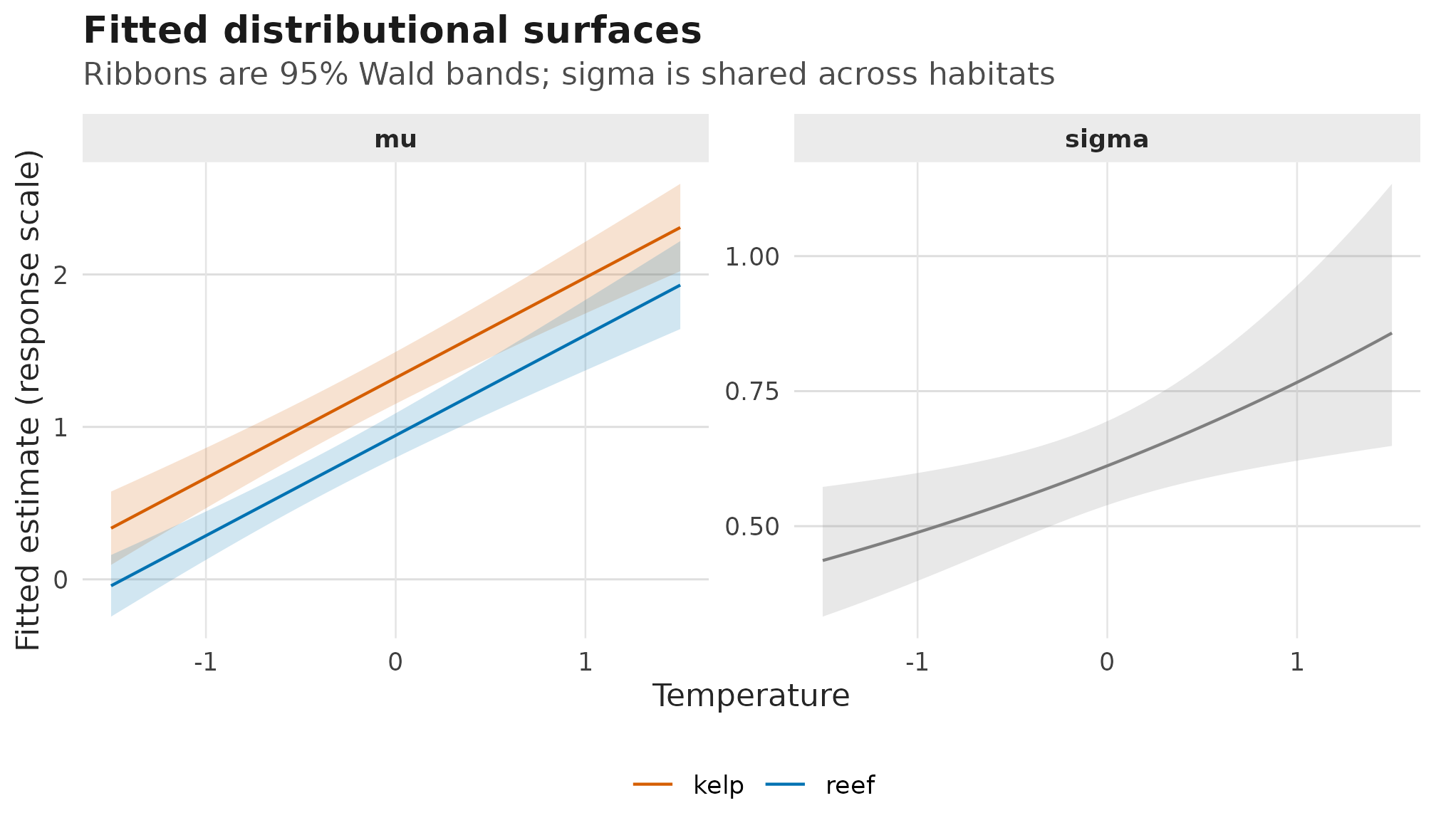
Fitted response-scale mu and sigma surfaces
from predict_parameters(); ribbons are 95% Wald confidence
bands, mu varies by habitat, and sigma is
shared because habitat is not in the scale formula.
For a discrete focal predictor, the same interval columns draw
interval bars rather than a ribbon. This example asks for 90% Wald
intervals, so the table records conf.level = 0.9 on rows
where conf.status = "wald":
habitat_plot_grid <- prediction_grid(
  fit,
  focal = "habitat",
  condition = list(temperature = 0)
)

pred_habitat <- predict_parameters(
  fit,
  newdata = habitat_plot_grid,
  dpar = "mu",
  conf.int = TRUE,
  conf.level = 0.90
)

unique(pred_habitat[, c(
  "dpar",
  "conf.status",
  "interval_source",
  "conf.level"
)])
#>   dpar conf.status interval_source conf.level
#> 1   mu        wald            wald        0.9

if (requireNamespace("ggplot2", quietly = TRUE)) {
  plot_parameter_surface(
    pred_habitat,
    x = "habitat",
    colour = "habitat",
    line = FALSE,
    facet = NULL
  ) +
    ggplot2::coord_flip() +
    workflow_habitat_scales() +
    workflow_theme() +
    ggplot2::labs(
      title = "Habitat contrast at average temperature",
      subtitle = "Points are fitted mu estimates; bars are 90% Wald intervals",
      x = NULL,
      y = "Fitted mean growth (mu)",
      colour = "Habitat"
    ) +
    ggplot2::guides(colour = "none")
}
#> Warning: No shared levels found between `names(values)` of the manual scale and the
#> data's fill values.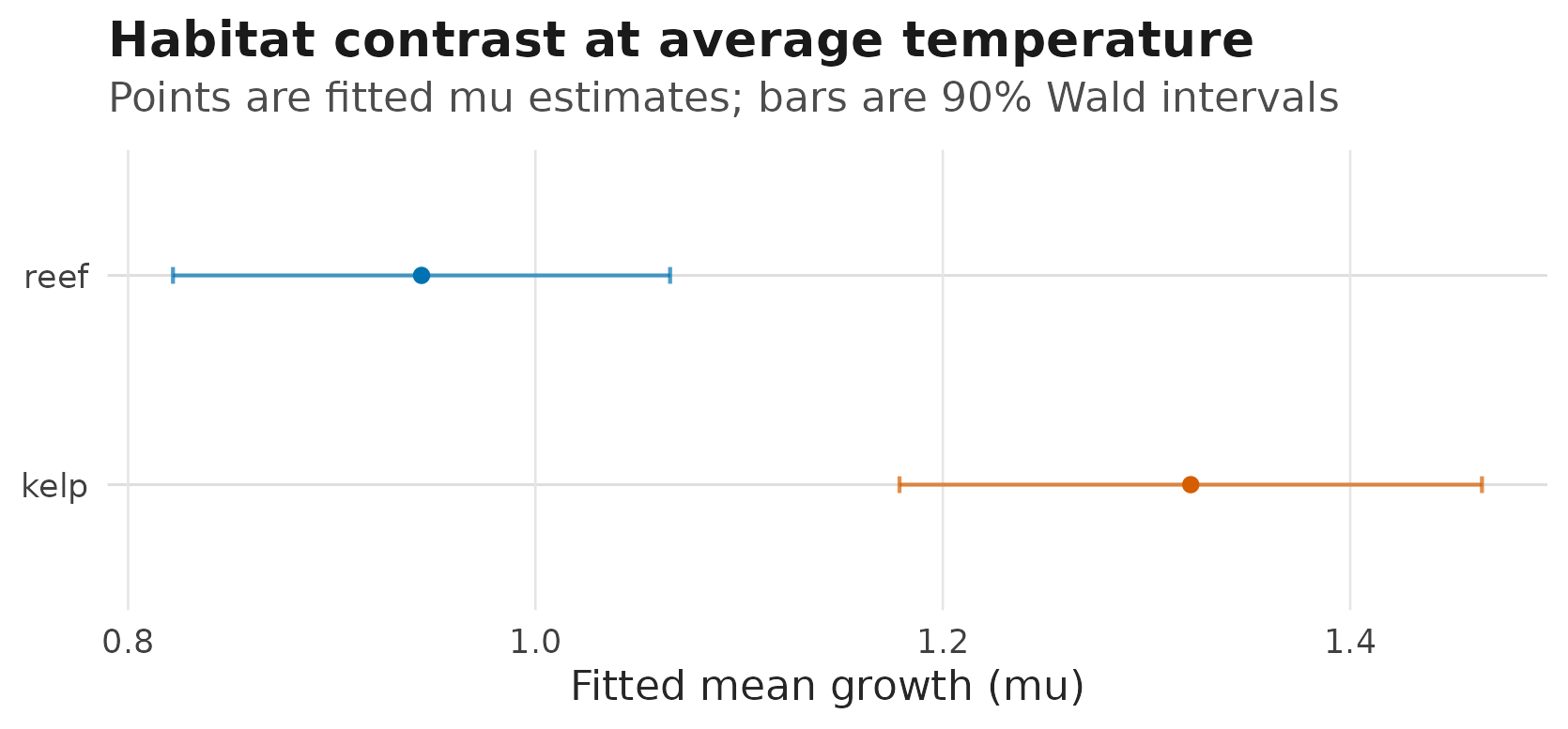
Fitted habitat-level mu estimates at temperature zero;
horizontal intervals are 90% Wald confidence intervals requested from
predict_parameters().
Treat conf.level as the requested level for rows where
an interval was computed or attempted. It is not a success flag by
itself; read it together with conf.status and
interval_source.
The figure is a convenience layer, not a new estimand. Keep reference grids, marginalization choices, and interval sources visible instead of hiding those decisions inside a plot.
For reports, pair model surfaces with the raw response pattern. The raw-data panel uses the observed response scale:
if (requireNamespace("ggplot2", quietly = TRUE)) {
  ggplot2::ggplot(
    fish,
    ggplot2::aes(x = temperature, y = growth, colour = habitat)
  ) +
    ggplot2::geom_point(alpha = 0.68, size = 1.8) +
    workflow_habitat_scales() +
    ggplot2::labs(
      title = "Observed growth before fitting",
      subtitle = "Points are raw response values; no model interval is shown",
      x = "Temperature",
      y = "Observed growth",
      colour = "Habitat"
    ) +
    workflow_theme() +
    ggplot2::guides(
      colour = ggplot2::guide_legend(
        override.aes = list(alpha = 1, size = 3)
      )
    )
}
#> Warning: No shared levels found between `names(values)` of the manual scale and the
#> data's fill values.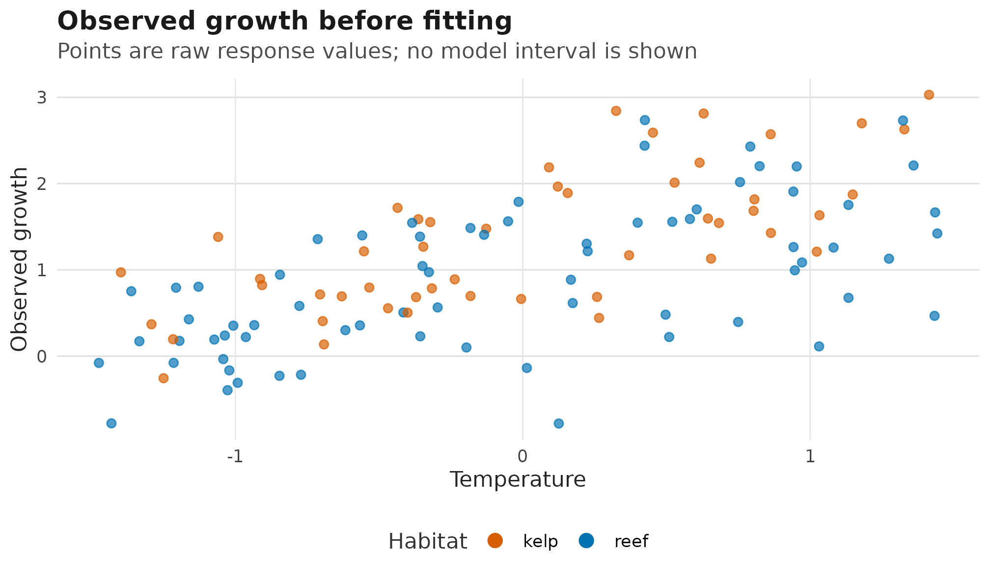
Raw response-scale growth observations by temperature and habitat, shown before the fitted distributional-parameter surfaces; no model uncertainty is plotted in this raw-data panel.
The fitted panels then use the prediction table. Keep mu
and sigma on their own y-axes because they are different
biological quantities. When a plot keeps one distributional parameter,
plot_parameter_surface() labels the y-axis with the
parameter and prediction scale. The bands in these panels come from the
Wald fixed-effect intervals in pred_temperature; if those
columns were absent or marked
interval_source = "not_available", the helper would draw
only lines and points:
if (requireNamespace("ggplot2", quietly = TRUE)) {
  plot_parameter_surface(
    pred_temperature,
    x = "temperature",
    colour = "habitat",
    dpar = "mu",
    facet = NULL,
    point = FALSE
  ) +
    workflow_habitat_scales() +
    workflow_theme() +
    ggplot2::labs(
      title = "Fitted mean growth by habitat",
      subtitle = "Ribbons are 95% Wald bands from predict_parameters()",
      x = "Temperature",
      y = "Fitted mean growth (mu)",
      colour = "Habitat",
      fill = "Habitat"
    )
}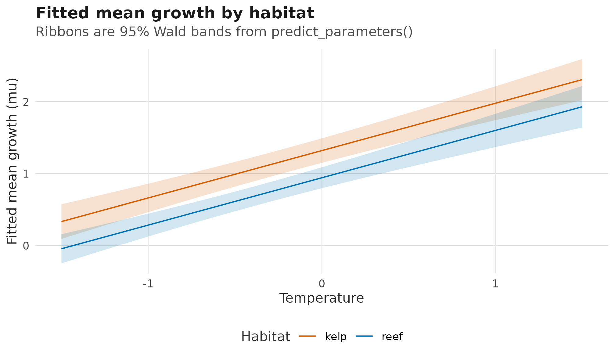
Fitted response-scale mu surface by habitat; ribbons are
95% Wald confidence bands from the prediction table.
Because sigma ~ temperature has no habitat term, the
sigma plot keeps one row per temperature. That avoids
drawing two identical habitat lines on top of each other.
if (requireNamespace("ggplot2", quietly = TRUE)) {
  pred_sigma_temperature <- pred_temperature[
    pred_temperature$dpar == "sigma" & pred_temperature$habitat == "reef",
  ]

  plot_parameter_surface(
    pred_sigma_temperature,
    x = "temperature",
    dpar = "sigma",
    facet = NULL,
    point = FALSE
  ) +
    workflow_theme() +
    ggplot2::labs(
      title = "Fitted residual SD over temperature",
      subtitle = "Ribbon is a 95% Wald band; habitat is not in sigma",
      x = "Temperature",
      y = "Fitted residual SD (sigma)"
    )
}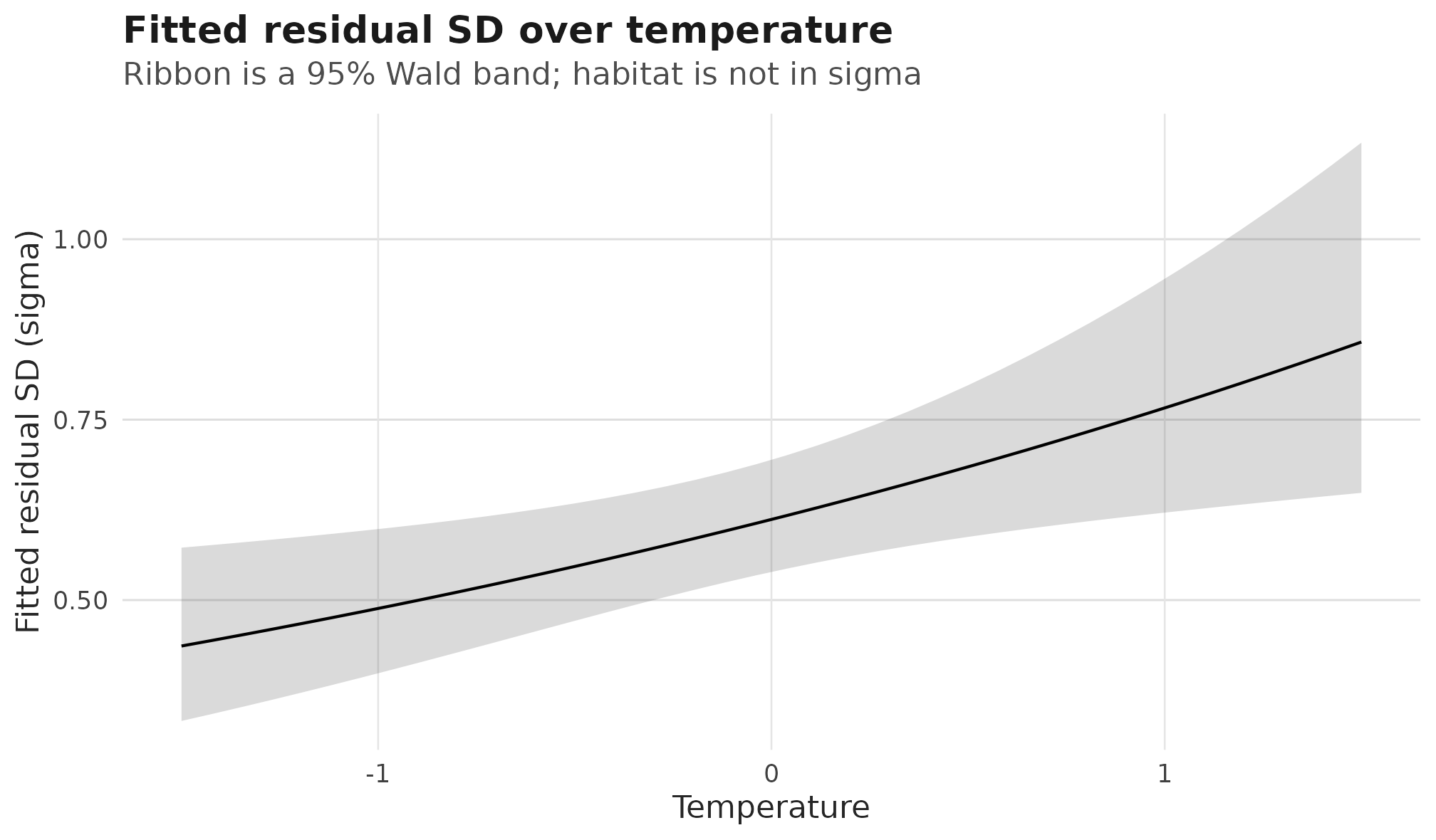
Fitted response-scale sigma surface over temperature; the
ribbon is a 95% Wald confidence band and only one band is drawn because
the scale formula has no habitat term.
Do not put raw growth points on the sigma
panel. Raw observations show the response; fitted sigma
shows the residual standard deviation implied by the model. The same
rule applies to uncertainty: draw a band only when the table names a
real interval source such as "wald" or
"profile".
For this Gaussian model, the response-scale sigma
predictions are residual standard deviations. The link-scale predictions
are the corresponding log-standard deviations. Report residual variance
as sigma(fit)^2 or
predict(fit, newdata = new_fish, dpar = "sigma")^2; do not
square the sigma coefficient, because coefficients are
fitted on the log-SD scale.
In meta-analytic Gaussian models with meta_V(V = V),
sigma(fit) still returns the modelled residual
heterogeneity scale. Simulation and Pearson residuals combine the known
sampling covariance with that residual scale internally.
Inspect residuals
Response residuals are observed minus fitted location:
Pearson residuals divide by the fitted observation scale:
head(residuals(fit, type = "pearson"))
#> [1] -0.2250209  0.8277852  0.5261116 -1.3961601 -1.2289053  1.2745290
For bivariate Gaussian fits,
residuals(fit, type = "pearson") returns a two-column
matrix whitened by the fitted sigma1, sigma2,
and residual correlation rho12.
Simulate from the fitted model
Simulation is a compact way to ask whether the fitted model generates data on the same scale as the observed response:
sims <- simulate(fit, nsim = 3, seed = 1)
head(sims)
#>        sim_1     sim_2      sim_3
#> 1 0.18565359 0.2407591  0.7956116
#> 2 1.71022792 2.5893123  2.3550726
#> 3 1.50558193 2.0179167  2.3792944
#> 4 1.70185743 0.7727547  0.4067588
#> 5 0.45297298 0.2427307  0.8607655
#> 6 0.03584287 0.7203782 -0.4908845
For this univariate model, the output has one column per simulated
data set. For bivariate Gaussian models, simulations are returned in
paired columns such as sim_1_y1 and
sim_1_y2.
A compact post-fit checklist
For routine fitted models, the post-fit loop is:
-
check_drm(fit)before interpreting estimates. -
summary(fit)for fixed effects, response-scale parameters, variance components, derived summaries, interval status, and the extractor to use next. -
profile_targets(fit)before asking for profile-likelihood intervals on fitted SD or correlation targets. -
predict(fit, dpar = ...)for fitted or new-data distributional parameters. -
residuals(fit, type = "pearson")to inspect standardized lack of fit. -
simulate(fit)to compare fitted-model behaviour with the observed data.
The same loop will extend as more families arrive. The parameter names change, but the discipline stays the same: check the fit, then interpret each distributional parameter on its own scale.
If any step in this loop becomes slow or memory-heavy as your data
grow, read Working with large data for
options such as keep_data, keep_model_frame,
and se = FALSE before abandoning the workflow above.
With a checked fit in hand, the next stage in the reader path is choosing a response family for your own data: continue with Which scale are you modelling? and Choosing response families.