Plot predicted distributional-parameter surfaces

plot_parameter_surface() is a small ggplot2 consumer for long tables returned by predict_parameters(). It does not fit a model, build a grid, compute predictions, compute confidence intervals, or choose an estimand. Build an explicit grid with prediction_grid() or another data-frame workflow first, then pass the resulting prediction table to this helper.

Usage

plot_parameter_surface(
  data,
  x,
  colour = NULL,
  group = NULL,
  facet = "dpar",
  dpar = NULL,
  type = NULL,
  line = TRUE,
  point = TRUE,
  interval = TRUE,
  ...
)

Arguments

data

A data frame returned by predict_parameters(), or a compatible long table with columns dpar, type, estimate, conf.status, and interval_source. If conf.low and conf.high are present, both must be numeric.

x

Character scalar naming the column to draw on the x-axis.

colour

Optional character scalar naming a column to map to colour.

group

Optional character scalar naming a column to group lines. If NULL, lines are grouped by dpar, colour, and facet columns when present.

facet

Optional character scalar naming a column to facet by. Use NULL to suppress faceting. The default facets by dpar.

dpar

Optional character vector of distributional parameters to keep.

type

Optional character vector of prediction scales to keep, such as "response" or "link".

line

Logical; draw lines through the estimates.

point

Logical; draw points at the estimates.

interval

Logical; draw finite conf.low/conf.high intervals when those columns are present and conf.status plus interval_source indicate that an interval was actually computed.

...

Reserved for future options.

Value

A ggplot object.

Details

The helper plots estimate against one supplied column. It expects the interval provenance columns created by predict_parameters(). When finite conf.low and conf.high columns are present and the provenance columns describe a real interval, it draws confidence bands for continuous x-values and interval bars for discrete x-values. Rows without finite supported bounds remain visible as point or line estimates only. When the filtered table contains a single distributional parameter, the y-axis label names that parameter and, when unique, the prediction scale.

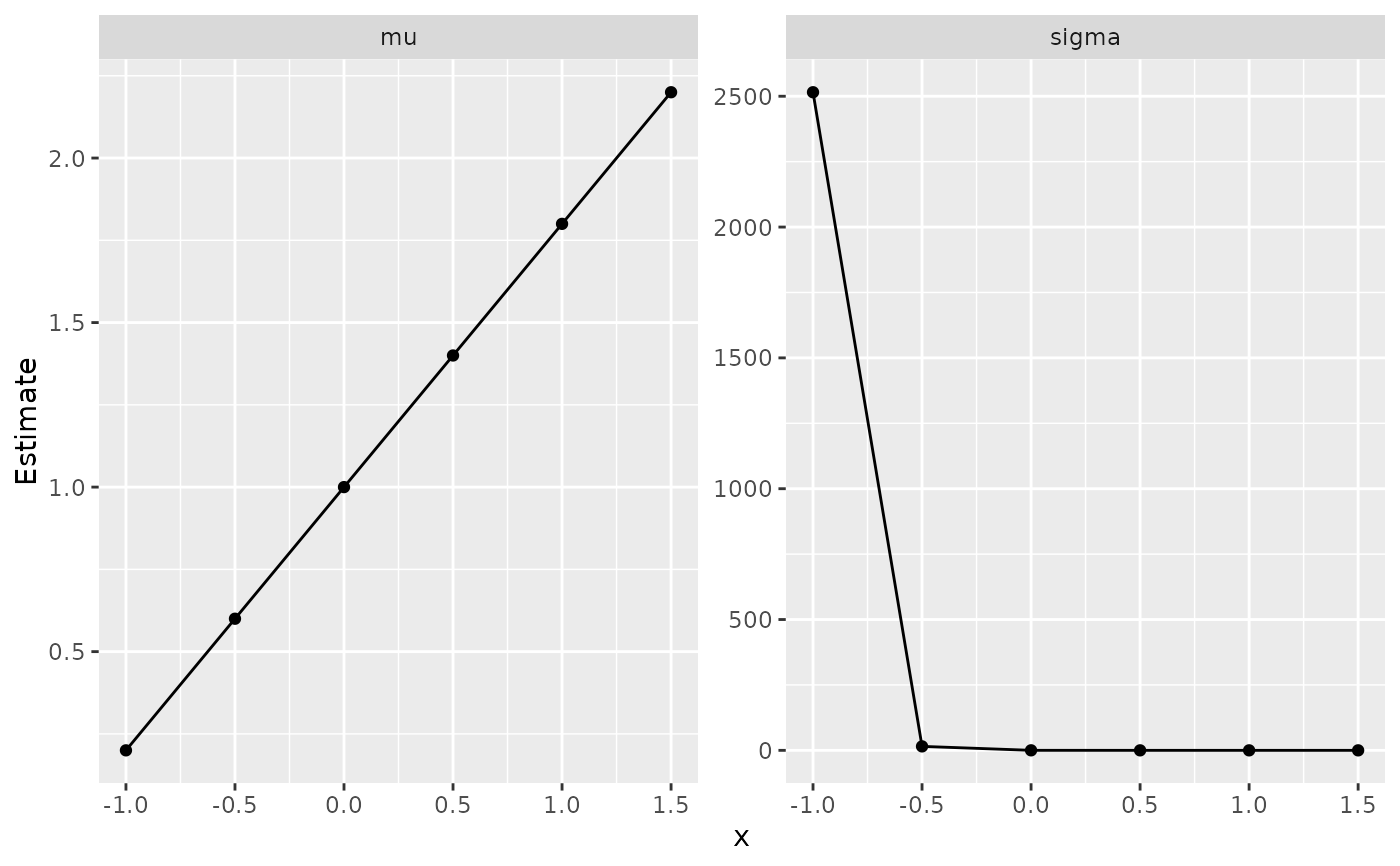
Examples

dat <- data.frame(
  y = c(0.2, 0.5, 1.1, 1.4, 1.8, 2.2),
  x = c(-1, -0.5, 0, 0.5, 1, 1.5)
)
fit <- drmTMB(bf(y ~ x, sigma ~ x), data = dat)
grid <- data.frame(x = seq(-1, 1.5, length.out = 6))
pred <- predict_parameters(
  fit,
  newdata = grid,
  dpar = c("mu", "sigma"),
  conf.int = TRUE
)
if (requireNamespace("ggplot2", quietly = TRUE)) {
  plot_parameter_surface(pred, x = "x")
}