Count abundance and extra zeros • drmTMB

Many ecological responses are counts: fledglings per nest, parasites per host, insects in a trap, or soil invertebrates in a quadrat. A Poisson model is the natural baseline, but it fixes the variance equal to the mean. The location-scale count question is sharper: do predictors change the expected abundance, the extra-Poisson variation around that abundance, or the chance of a separate structural zero? This tutorial assumes the location-scale reading pattern from When variance carries signal, Part 1 and extends it to a count mean and dispersion.

This article stays inside the currently implemented drmTMB count surface: univariate NB2 models, fixed-effect zero-inflated NB2 models, ordinary Poisson and NB2 mu random-effect paths, and the first ordinary Poisson/NB2 q=1 structured mu intercept-plus-one-slope routes for phylo(), spatial(), animal(), and relmat(). Ordinary NB2 also has a first grouped overdispersion path in sigma and exact q1 structured sigma intercept-plus-one-slope routes for those four providers at recovery grade. The worked example below remains fixed-effect so the mean, overdispersion, and structural-zero pieces are easy to read before adding grouped or structured log-mean effects, grouped overdispersion, or the narrow structured-overdispersion routes.

The source motivation comes from Nakagawa et al. (2026), who use location-scale models to discuss heteroscedasticity in continuous, count, and proportion data. Their count section highlights negative-binomial models for fledglings, insect colony size, parasites, and soil invertebrates, and it separates overdispersion from structural-zero processes. drmTMB uses the same scientific split, but reports the NB2 scale as public sigma rather than the native size or precision parameter often written as theta.

Model Equation And Syntax

For an overdispersed count model, nbinom2() uses

$\begin{aligned} Y_i \mid \mu_i, \sigma_i &\sim \operatorname{NB2}(\mu_i, \text{size}_i),\\ \log(\mu_i) &= \log(E_i) + \beta_0 + \beta_1 \text{restored}_i + \beta_2 \text{moisture}_i,\\ \log(\sigma_i) &= \gamma_0 + \gamma_1 \text{restored}_i,\\ \text{size}_i &= 1 / \sigma_i^2,\\ E[Y_i] &= \mu_i,\\ \operatorname{Var}(Y_i) &= \mu_i + \sigma_i^2\mu_i^2. \end{aligned}$

The matching drmTMB syntax is:

drmTMB(
  bf(
    springtails ~ habitat + moisture + offset(log(trap_nights)),
    sigma ~ habitat
  ),
  family = nbinom2(),
  data = soil_counts
)

Read each parameter before interpreting the fitted model:

Symbol or syntax	Meaning	In the soil-invertebrate example
$Y_i$ , `springtails`	observed non-negative integer count	springtails found in trap $i$
$E_i$ , `trap_nights`	sampling effort exposure	number of nights the trap was active
`offset(log(trap_nights))`	forces expected count to scale with effort	estimates abundance rate per trap night
$\mu_i$ , `mu`	expected count after accounting for effort	expected springtail abundance in a trap
$\boldsymbol{\beta}_{\mu}$	location coefficients on the log mean scale	habitat and moisture effects on expected abundance
$\sigma_i$ , `sigma`	NB2 extra-Poisson scale	variation beyond the Poisson expectation
$\boldsymbol{\beta}_{\sigma}$	scale coefficients on the log `sigma` scale	habitat effects on extra-Poisson variation
$\text{size}_i$ , `theta` in some papers	native NB2 size or precision	`size_i = 1 / sigma_i^2`, so larger `sigma` means smaller `size`

The sigma slope is a variability slope. If gamma_1 is the restored-habitat coefficient, then

$\frac{\sigma_\text{restored}}{\sigma_\text{degraded}} = \exp(\gamma_1), \qquad \frac{\sigma_\text{restored}^2}{\sigma_\text{degraded}^2} = \exp(2\gamma_1).$

If a paper reports the native NB2 parameter $\theta_i = 1 / \sigma_i^2$ , the direction reverses:

$\frac{\theta_\text{restored}}{\theta_\text{degraded}} = \exp(-2\gamma_1).$

That reversal is why the tutorial keeps saying sigma: in drmTMB, larger sigma always means more modelled variation for this family.

A Soil-Invertebrate Example

Suppose springtails are counted from soil traps in degraded and restored grassland plots. Restoration may increase average abundance, but restored plots may also be more patchy while litter and vegetation structure re-establish. A few bare-soil microsites may be true absences where springtails are not available to be trapped.

This transparent simulation gives us known structure before fitting:

set.seed(106)
n <- 360
soil_counts <- data.frame(
  habitat = factor(
    rep(c("degraded", "restored"), each = n / 2),
    levels = c("degraded", "restored")
  ),
  surface = factor(
    sample(c("litter", "bare"), n, replace = TRUE, prob = c(0.72, 0.28)),
    levels = c("litter", "bare")
  ),
  moisture = as.numeric(scale(runif(n, 0.15, 0.95))),
  trap_nights = sample(2:5, n, replace = TRUE)
)

restored <- as.numeric(soil_counts$habitat == "restored")
bare <- as.numeric(soil_counts$surface == "bare")

rate <- exp(log(2.4) + 0.35 * restored + 0.30 * soil_counts$moisture)
mu <- soil_counts$trap_nights * rate
sigma_nb2 <- exp(-0.75 + 0.40 * restored)
zi <- plogis(-3.2 + 1.6 * bare - 0.25 * restored)

structural_zero <- runif(n) < zi
soil_counts$springtails <- ifelse(
  structural_zero,
  0L,
  rnbinom(n, size = 1 / sigma_nb2^2, mu = mu)
)

head(soil_counts)
#>    habitat surface   moisture trap_nights springtails
#> 1 degraded  litter -1.1665372           3           1
#> 2 degraded    bare  1.5939065           4           4
#> 3 degraded  litter  0.4203317           5          14
#> 4 degraded  litter  0.6364855           5           7
#> 5 degraded  litter  1.0379937           4           5
#> 6 degraded  litter -1.4584601           2           3

Start with the NB2 location-scale model before adding a structural-zero submodel:

fit_nb2 <- drmTMB(
  bf(
    springtails ~ habitat + moisture + offset(log(trap_nights)),
    sigma ~ habitat
  ),
  family = nbinom2(),
  data = soil_counts
)

Run diagnostics before interpreting coefficients:

check_drm(fit_nb2)
#> <drm_check: 12 checks>
#> ok: 12; notes: 0; warnings: 0; errors: 0
#>                      check status
#>      optimizer_convergence     ok
#>           optimizer_budget     ok
#>           finite_objective     ok
#>      logsigma_clamp_active     ok
#>             fixed_gradient     ok
#>            sdreport_status     ok
#>  hessian_positive_definite     ok
#>     standard_errors_finite     ok
#>   standard_errors_inflated     ok
#>               dropped_rows     ok
#>             positive_scale     ok
#>   fixed_effect_design_size     ok
#>                                                                                   value
#>                                                                                       0
#>                                                 iterations=17; function=29; gradient=17
#>                                                                                   1130.
#>                                                                                    <NA>
#>                                                     max=0.0007830; component=beta_mu[3]
#>                                                                                      ok
#>                                                                                    TRUE
#>                                                                  range=[0.04334,0.1013]
#>                                          n_inflated=0; max_se=0.1013; median_se=0.07791
#>                                                                     nobs=360; dropped=0
#>                                                                              min=0.6499
#>  total_mb=0.06026; max_cols=3; largest=mu; largest_class=matrix; largest_density=0.8333
#>                                                                              message
#>                                                        nlminb convergence code is 0.
#>  Optimizer evaluation counts recorded; no eval.max or iter.max control was supplied.
#>                                             Objective and log-likelihood are finite.
#>                                   The log(sigma) clamp is not active at the optimum.
#>        Maximum absolute fixed gradient is <= 0.001; largest component is beta_mu[3].
#>                                              TMB::sdreport() completed successfully.
#>                                        sdreport reports a positive-definite Hessian.
#>                                         All fixed-effect standard errors are finite.
#>                   No fixed-effect standard error is inflated relative to the others.
#>                   No rows were dropped by model-frame or known-covariance filtering.
#>                                     All fitted scale values are finite and positive.
#>                          Dense fixed-effect design matrices are modest for this fit.

The NB2 fit answers two questions. The mu coefficients describe abundance rates, because the offset has already accounted for trap effort. The sigma coefficients describe extra-Poisson variation in the count component:

coef(fit_nb2, "mu")
#>     (Intercept) habitatrestored        moisture 
#>       0.7603134       0.3511186       0.2422656
coef(fit_nb2, "sigma")
#>     (Intercept) habitatrestored 
#>      -0.4309409       0.2758195

sigma_ratio <- exp(coef(fit_nb2, "sigma")["habitatrestored"])
c(
  sigma_ratio_restored_vs_degraded = sigma_ratio,
  variance_multiplier_at_same_mu = sigma_ratio^2
)
#> sigma_ratio_restored_vs_degraded.habitatrestored 
#>                                         1.317610 
#>   variance_multiplier_at_same_mu.habitatrestored 
#>                                         1.736096

The second value is the multiplier on the quadratic extra-Poisson part $\sigma_i^2\mu_i^2$ when two traps have the same expected count. It is not the full variance ratio whenever $\mu_i$ also changes, because NB2 variance contains both $\mu_i$ and $\sigma_i^2\mu_i^2$ .

When Zeros Are A Separate Process

The paper example of soil invertebrates in patchy habitats maps naturally to a zero-inflated count model. Bare-soil microsites can be true absences, while litter microsites can still produce ordinary sampling zeros from the NB2 count component. Add a zi formula when the biological question needs that split:

$\begin{aligned} \Pr(Y_i = 0) &= \pi_i + (1 - \pi_i)\Pr_{\operatorname{NB2}}(0 \mid \mu_i,\sigma_i),\\ \Pr(Y_i = k > 0) &= (1 - \pi_i)\Pr_{\operatorname{NB2}}(k \mid \mu_i,\sigma_i),\\ \operatorname{logit}(\pi_i) &= \delta_0 + \delta_1 \text{bare}_i,\\ \operatorname{Var}(Y_i) &= (1 - \pi_i)(\mu_i + \sigma_i^2\mu_i^2) + \pi_i(1 - \pi_i)\mu_i^2. \end{aligned}$

In this equation, $\pi_i$ is the structural-zero probability. It is not a scale parameter and should not be interpreted as overdispersion.

fit_zinb2 <- drmTMB(
  bf(
    springtails ~ habitat + moisture + offset(log(trap_nights)),
    sigma ~ habitat,
    zi ~ surface
  ),
  family = nbinom2(),
  data = soil_counts
)

check_drm(fit_zinb2)
#> <drm_check: 12 checks>
#> ok: 12; notes: 0; warnings: 0; errors: 0
#>                      check status
#>      optimizer_convergence     ok
#>           optimizer_budget     ok
#>           finite_objective     ok
#>      logsigma_clamp_active     ok
#>             fixed_gradient     ok
#>            sdreport_status     ok
#>  hessian_positive_definite     ok
#>     standard_errors_finite     ok
#>   standard_errors_inflated     ok
#>               dropped_rows     ok
#>             positive_scale     ok
#>   fixed_effect_design_size     ok
#>                                                                                   value
#>                                                                                       0
#>                                                 iterations=31; function=41; gradient=32
#>                                                                                   1105.
#>                                                                                    <NA>
#>                                                 max=0.00004223; component=beta_sigma[2]
#>                                                                                      ok
#>                                                                                    TRUE
#>                                                                  range=[0.03636,0.4202]
#>                                          n_inflated=0; max_se=0.4202; median_se=0.09309
#>                                                                     nobs=360; dropped=0
#>                                                                              min=0.4904
#>  total_mb=0.08898; max_cols=3; largest=mu; largest_class=matrix; largest_density=0.8333
#>                                                                              message
#>                                                        nlminb convergence code is 0.
#>  Optimizer evaluation counts recorded; no eval.max or iter.max control was supplied.
#>                                             Objective and log-likelihood are finite.
#>                                   The log(sigma) clamp is not active at the optimum.
#>     Maximum absolute fixed gradient is <= 0.001; largest component is beta_sigma[2].
#>                                              TMB::sdreport() completed successfully.
#>                                        sdreport reports a positive-definite Hessian.
#>                                         All fixed-effect standard errors are finite.
#>                   No fixed-effect standard error is inflated relative to the others.
#>                   No rows were dropped by model-frame or known-covariance filtering.
#>                                     All fitted scale values are finite and positive.
#>                          Dense fixed-effect design matrices are modest for this fit.

The zi coefficients are on the log-odds scale. Prediction gives the structural-zero probability on the response scale:

coef(fit_zinb2, "zi")
#> (Intercept) surfacebare 
#>   -2.786077    1.215586

zero_grid <- data.frame(
  habitat = factor(c("degraded", "degraded"), levels = levels(soil_counts$habitat)),
  surface = factor(c("litter", "bare"), levels = levels(soil_counts$surface)),
  moisture = 0,
  trap_nights = 3
)

data.frame(
  surface = zero_grid$surface,
  structural_zero_probability = predict(fit_zinb2, newdata = zero_grid, dpar = "zi")
)
#>   surface structural_zero_probability
#> 1  litter                  0.05808118
#> 2    bare                  0.17214634

For the fitted zero-inflated model, predict(fit_zinb2, dpar = "mu") returns the conditional NB2 count mean, sigma(fit_zinb2) returns the conditional NB2 overdispersion scale, and fitted(fit_zinb2) returns the unconditional response mean $(1 - \pi_i)\mu_i$ :

new_traps <- data.frame(
  habitat = factor(c("degraded", "restored"), levels = levels(soil_counts$habitat)),
  surface = factor(c("litter", "litter"), levels = levels(soil_counts$surface)),
  moisture = c(0, 0),
  trap_nights = c(3, 3)
)

mu_hat <- predict(fit_zinb2, newdata = new_traps, dpar = "mu")
sigma_hat <- predict(fit_zinb2, newdata = new_traps, dpar = "sigma")
zi_hat <- predict(fit_zinb2, newdata = new_traps, dpar = "zi")

data.frame(
  habitat = new_traps$habitat,
  conditional_mean = mu_hat,
  sigma = sigma_hat,
  structural_zero_probability = zi_hat,
  unconditional_mean = (1 - zi_hat) * mu_hat,
  unconditional_variance =
    (1 - zi_hat) * (mu_hat + sigma_hat^2 * mu_hat^2) +
      zi_hat * (1 - zi_hat) * mu_hat^2
)
#>    habitat conditional_mean     sigma structural_zero_probability
#> 1 degraded         6.924234 0.4903942                  0.05808118
#> 2 restored        10.124436 0.6257923                  0.05808118
#>   unconditional_mean unconditional_variance
#> 1           6.522067               20.00548
#> 2           9.536397               52.95495

library(ggplot2)

count_plot_grid <- expand.grid(
  habitat = factor(levels(soil_counts$habitat), levels = levels(soil_counts$habitat)),
  surface = factor(levels(soil_counts$surface), levels = levels(soil_counts$surface))
)
count_plot_grid$moisture <- 0
count_plot_grid$trap_nights <- 3
count_plot_grid$conditional_mean <- predict(
  fit_zinb2,
  newdata = count_plot_grid,
  dpar = "mu"
)
count_plot_grid$sigma <- predict(fit_zinb2, newdata = count_plot_grid, dpar = "sigma")
count_plot_grid$structural_zero_probability <- predict(
  fit_zinb2,
  newdata = count_plot_grid,
  dpar = "zi"
)
count_plot_grid$unconditional_mean <-
  (1 - count_plot_grid$structural_zero_probability) *
  count_plot_grid$conditional_mean
count_plot_grid$row_label <- paste(count_plot_grid$habitat, count_plot_grid$surface)
count_plot_long <- rbind(
  data.frame(
    count_plot_grid[c("habitat", "row_label")],
    component = "Conditional mean",
    value = count_plot_grid$conditional_mean
  ),
  data.frame(
    count_plot_grid[c("habitat", "row_label")],
    component = "Unconditional mean",
    value = count_plot_grid$unconditional_mean
  ),
  data.frame(
    count_plot_grid[c("habitat", "row_label")],
    component = "NB2 sigma",
    value = count_plot_grid$sigma
  ),
  data.frame(
    count_plot_grid[c("habitat", "row_label")],
    component = "Structural-zero probability",
    value = count_plot_grid$structural_zero_probability
  )
)
count_plot_long$component <- factor(
  count_plot_long$component,
  levels = c(
    "Conditional mean",
    "Unconditional mean",
    "NB2 sigma",
    "Structural-zero probability"
  )
)
count_plot_long$row_label <- factor(
  count_plot_long$row_label,
  levels = rev(unique(count_plot_grid$row_label))
)

ggplot(count_plot_long, aes(value, row_label, colour = habitat)) +
  geom_point(size = 2.7) +
  facet_wrap(~component, scales = "free_x", ncol = 2) +
  scale_colour_manual(values = c("degraded" = "#D55E00", "restored" = "#009E73")) +
  labs(
    title = "Zero-inflated counts have several fitted pieces",
    subtitle = "Facets keep count means, NB2 sigma, and structural-zero probabilities separate",
    x = "Response-scale fitted value",
    y = NULL,
    colour = "Habitat"
  ) +
  theme_minimal(base_size = 11) +
  theme(
    panel.grid.minor = element_blank(),
    panel.grid.major.y = element_blank(),
    legend.position = "bottom",
    plot.title = element_text(face = "bold"),
    plot.subtitle = element_text(colour = "grey30"),
    strip.text = element_text(face = "bold")
  )

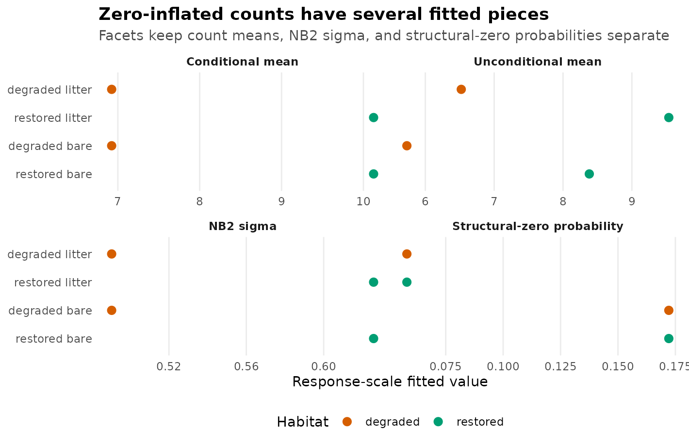
Faceted point plot for the zero-inflated NB2 soil-count example. Separate facets show conditional expected counts, unconditional expected counts, NB2 extra-Poisson sigma, and structural-zero probabilities for habitat and surface combinations.

Response-scale model parts for the zero-inflated NB2 example. Points show fitted conditional counts, unconditional counts, NB2 extra-Poisson scale, and structural-zero probabilities on separate facets with their own x scales. No interval bars are drawn because this figure compares fitted components, not confidence intervals.

Use AIC only as one check, not as a substitute for the design story. A zero-inflated model needs a plausible structural-zero process such as bare soil, unsuitable host tissue, unsurveyable habitat, or true absence.

AIC(fit_nb2, fit_zinb2)
#>   df      AIC
#> 1  5 2270.559
#> 2  7 2223.058

Current Boundary

The implemented count path is still intentionally narrow. Fixed-effect Poisson, NB2, zero-inflated Poisson, zero-inflated NB2, zero-truncated NB2, and hurdle NB2 models are fitted. Ordinary non-zero-inflated Poisson and NB2 mu models can also fit unlabelled random intercepts and independent numeric random slopes such as (1 | site) and (0 + effort | site). The first structured count routes are ordinary Poisson and ordinary NB2 q=1 structured mu intercept-plus-one-slope terms via phylo(1 + x | species, tree = tree), spatial(), animal(), and relmat(), one at a time, on the log-mean scale (recovery grade – trust the point estimate, not the interval). Ordinary NB2 also fits sigma ~ z + (1 | id) as a grouped overdispersion random intercept on the log-sigma scale and the same four q=1 structured intercept-plus-one-slope shapes in sigma, separately from mu, at recovery grade. Zero-inflated, hurdle, and truncated scale-side count routes remain fixed-effect only.

drmTMB(
  bf(count ~ habitat + offset(log(effort)), sigma ~ habitat, zi ~ surface),
  family = nbinom2(),
  data = dat
)

For ordinary non-zero-inflated NB2 models, the fitted q1 structured boundary is wider than an intercept: unlabelled phylo(), spatial(), animal(), and relmat() intercept-plus-one-slope terms fit in mu, and the exact same four providers fit q1 structured sigma intercept-plus-one-slope routes at recovery grade. For example, the two separate fitted shapes are:

bf(count ~ habitat + phylo(1 + x | species, tree = tree), sigma ~ z)
bf(count ~ habitat, sigma ~ z + phylo(1 + x | species, tree = tree))

The structured-sigma rows do not yet have interval or coverage promotion. Pure, labelled, or multiple structured slopes and richer count covariance remain planned.

Hurdle NB2 has one separate diagnostic-only structured probability route: an unlabelled q=1 relatedness intercept in hu, supplied by K or Q:

bf(count ~ habitat, sigma ~ treatment,
  hu ~ relmat(1 | id, K = K))

Treat this exact route as diagnostic-only fit/extractor evidence. It does not establish point-estimate recovery, intervals, coverage, slopes, labels, or other structured providers.

Zero-inflated Poisson likewise has one diagnostic-only probability-component gate, zi ~ spatial(1 | id, coords = coords), for a q=1 structured intercept. It confirms fit/extractor feasibility but does not establish point-estimate recovery, NB2 zi, spatial slopes, labels, intervals, or coverage.

Two separate gates keep zero inflation fixed and put one q=1 spatial intercept in the count mean. The exact diagnostic-only formulas are bf(count ~ habitat + spatial(1 | site, coords = coords), zi ~ 1) for Poisson and bf(count ~ habitat + spatial(1 | site, coords = coords), sigma ~ 1, zi ~ 1) for NB2. Both confirm only local fit/extractor feasibility. These two gates do not establish point-estimate recovery, intervals, or coverage, and neither is evidence for a random effect in zi.

Do not teach the following as fitted count examples yet:

correlated or labelled NB2 mu random-slope blocks;
ordinary NB2 sigma random slopes, labelled blocks, richer structured effects beyond the exact q1 routes, or zi random effects beyond the exact Poisson q=1 spatial-zi intercept;
random effects in zero-inflated Poisson beyond the exact q=1 spatial zi intercept; fixed-zi Poisson or NB2 spatial-mu routes beyond the two exact diagnostic-only q=1 intercept gates; and other zero-inflated NB2, truncated NB2, or hurdle NB2 count-mu components;
sd(group) ~ ... random-effect scale models;
meta_V(V = V) or deprecated meta_known_V(V = V) with counts;
zero-inflated structured count models beyond the exact q=1 Poisson zi ~ spatial() intercept and the exact diagnostic-only fixed-zi Poisson and NB2 mu ~ spatial() intercepts, and hurdle structured routes beyond the exact q=1 hu ~ relmat(K/Q) intercept; pure, labelled, or multiple structured count slopes; simultaneous structured count types beyond the exact crossed NB2 mu ~ spatial() + relmat() recovery-only gate; and labelled structured count covariance;
richer or labelled NB2 phylogenetic slopes, richer NB2 sigma phylogeny, and zero-inflated NB2 phylogeny;
pure, labelled, or multiple phylogenetic count slopes or labelled q2/q4 phylogenetic count covariance;
bivariate or mixed-response count models such as family = c(gaussian(), nbinom2());
COM-Poisson underdispersion models.

Those are useful future routes, but each needs its own likelihood path, simulation recovery, diagnostics, and a source-map update before it becomes tutorial syntax.