This gallery shows the kinds of figures drmTMB users can
build for model interpretation, uncertainty display, distributional
adequacy checking, fitted interactions, correlation summaries, and later
simulation diagnostics. Between them the panels exercise all six public
plotting functions: plot_parameter_surface(),
worm_plot(), qq_plot(),
centile_chart(), plot_corpairs(), and the
plot() method for profile objects. It is different from the
internal count-pilot diagnostics used while developing the first
Poisson/NB2 simulation plumbing. The panels apply the same
location-scale reading pattern taught in the family tutorials, such as
When variance carries signal, Part 1;
read one of those first for the modelling context behind a given
figure.
The examples here use small simulated data so the page can build quickly. They are meant to show figure patterns, not biological conclusions. The interaction figures deliberately keep three pieces visible: the observed data, the fitted surface or cell means, and the conditioning values used to make the display. Across the gallery, the right display depends on the figure’s job. Raw data are often warranted and sometimes preferred, especially when the reader needs to see sample grain, spread, outliers, or repeated-measures structure. When the figure makes an inferential claim, pair the estimate with uncertainty if the fitted object or simulation output provides it: a slope estimate can be a line with a confidence band, a cell mean can be a point with an interval, and selected row-wise summaries can use Confidence Eyes. When uncertainty is unavailable or outside the current support boundary, the figure should say so rather than drawing a decorative interval.
The examples keep consistency within a figure family rather than forcing one geometry everywhere. Raw-data displays, model-surface displays, row-wise interval summaries, simulation summaries, and support-boundary strips each use their own grammar because they answer different reader questions.
library(drmTMB)
#>
#> Attaching package: 'drmTMB'
#> The following object is masked from 'package:base':
#>
#>     beta
library(ggplot2)

theme_drmtmb_gallery <- function() {
  theme_minimal(base_size = 10.5) +
    theme(
      panel.grid.minor = element_blank(),
      panel.grid.major.x = element_blank(),
      axis.title = element_text(size = 10.5, colour = "grey15"),
      axis.text = element_text(size = 9.5, colour = "grey30"),
      plot.title.position = "plot",
      plot.title = element_text(size = 12.5, face = "bold"),
      plot.subtitle = element_text(size = 10.2, colour = "grey30"),
      strip.text = element_text(size = 10, face = "bold"),
      legend.position = "bottom",
      legend.title = element_text(colour = "grey20"),
      legend.text = element_text(size = 9.5),
      legend.key.width = grid::unit(1.0, "lines"),
      plot.margin = margin(5.5, 9, 5.5, 5.5)
    )
}
theme_confidence_eye <- function() {
  theme_drmtmb_gallery() +
    theme(
      axis.line.x = element_line(colour = "grey35", linewidth = 0.35),
      axis.ticks.x = element_line(colour = "grey35", linewidth = 0.35),
      axis.ticks.length.x = grid::unit(3, "pt"),
      panel.grid.major.x = element_line(colour = "grey88", linewidth = 0.35),
      panel.grid.major.y = element_blank(),
      panel.grid.minor = element_blank()
    )
}
theme_point_interval_gallery <- function() {
  theme_drmtmb_gallery() +
    theme(
      panel.grid.major.x = element_line(colour = "grey90", linewidth = 0.35),
      panel.grid.major.y = element_line(colour = "grey92", linewidth = 0.35),
      axis.title = element_text(size = 10, colour = "grey15"),
      axis.text = element_text(size = 10, colour = "grey30"),
      plot.title = element_text(size = 12, face = "bold"),
      plot.subtitle = element_text(size = 10, colour = "grey30"),
      plot.margin = margin(5.5, 10, 5.5, 5.5)
    )
}

gallery_colours <- c(
  blue = "#0072B2",
  green = "#009E73",
  orange = "#D55E00",
  yellow = "#E69F00",
  pink = "#CC79A7",
  sky = "#56B4E9",
  charcoal = "#4D4D4D"
)
gallery_colour <- function(name) unname(gallery_colours[name])

habitat_palette <- c(
  "reef" = gallery_colour("blue"),
  "kelp" = gallery_colour("orange")
)
season_palette <- c(
  "dry" = gallery_colour("blue"),
  "wet" = gallery_colour("yellow")
)
surface_palette <- c(
  "Gaussian location-scale" = gallery_colour("blue"),
  "Proportion" = gallery_colour("green"),
  "Count" = gallery_colour("pink")
)
make_confidence_eye_distribution <- function(
  parameter,
  estimate,
  std_error,
  transform = c("identity", "exp", "tanh"),
  null_value = 0,
  level = 0.95,
  n = 500
) {
  transform <- match.arg(transform)
  cutoff <- 0.5 * qchisq(level, df = 1)
  theta <- seq(
    estimate - sqrt(2 * cutoff) * std_error,
    estimate + sqrt(2 * cutoff) * std_error,
    length.out = n
  )
  value <- switch(
    transform,
    identity = theta,
    exp = exp(theta),
    tanh = tanh(theta)
  )
  height <- pmax(cutoff - 0.5 * ((theta - estimate) / std_error)^2, 0) /
    cutoff
  data.frame(
    parameter = parameter,
    theta = theta,
    value = value,
    cdf = pnorm(theta, mean = estimate, sd = std_error),
    height = height,
    null_value = switch(
      transform,
      identity = null_value,
      exp = exp(null_value),
      tanh = tanh(null_value)
    ),
    estimate_value = switch(
      transform,
      identity = estimate,
      exp = exp(estimate),
      tanh = tanh(estimate)
    )
  )
}
guard_rho <- function(x) pmin(pmax(x, -0.999999), 0.999999)
response_scale_se_to_log_se <- function(estimate, std_error) {
  ifelse(is.finite(estimate) & estimate > 0, std_error / estimate, NA_real_)
}
response_scale_se_to_z_se <- function(estimate, std_error) {
  rho <- guard_rho(estimate)
  std_error / pmax(1 - rho^2, .Machine$double.eps)
}

wrap_subtitle <- function(p, width = 78) {
  subtitle <- p$labels$subtitle
  if (is.null(subtitle)) {
    return(p)
  }
  p + labs(subtitle = paste(strwrap(subtitle, width = width), collapse = "\n"))
}

scale_drmtmb_colour <- scale_colour_manual(
  values = habitat_palette,
  limits = names(habitat_palette)
)
scale_drmtmb_fill <- scale_fill_manual(
  values = habitat_palette,
  limits = names(habitat_palette)
)
Fitted mean with a confidence band
Start with the figure most readers expect: raw observations, fitted mean, and a 95% confidence band on the response scale. This example is also a categorical-by-continuous interaction: the temperature slope differs by habitat.
set.seed(2591)
n <- 160
habitat_levels <- c("reef", "kelp")
fish <- data.frame(
  temperature = runif(n, -1.6, 1.6),
  habitat = factor(
    sample(habitat_levels, n, replace = TRUE),
    levels = habitat_levels
  )
)
eta_mu <- 0.4 +
  0.7 * fish$temperature +
  0.35 * (fish$habitat == "kelp") +
  0.18 * fish$temperature * (fish$habitat == "kelp")
eta_sigma <- -0.55 + 0.35 * fish$temperature
fish$growth <- rnorm(n, mean = eta_mu, sd = exp(eta_sigma))

fit_growth <- drmTMB(
  bf(growth ~ temperature * habitat, sigma ~ temperature),
  family = gaussian(),
  data = fish
)

grid_growth <- expand.grid(
  temperature = seq(-1.6, 1.6, length.out = 80),
  habitat = levels(fish$habitat)
)
pred_growth <- predict_parameters(
  fit_growth,
  newdata = grid_growth,
  dpar = c("mu", "sigma"),
  conf.int = TRUE
)
pred_growth$panel <- factor(
  ifelse(
    pred_growth$dpar == "mu",
    "Expected growth (mu)",
    "Residual SD (sigma)"
  ),
  levels = c("Expected growth (mu)", "Residual SD (sigma)")
)

pred_mu <- pred_growth[pred_growth$dpar == "mu", , drop = FALSE]
pred_sigma <- pred_growth[pred_growth$dpar == "sigma", , drop = FALSE]

ggplot(fish, aes(temperature, growth, colour = habitat)) +
  geom_point(alpha = 0.35, size = 1.4) +
  geom_ribbon(
    data = pred_mu,
    aes(
      x = temperature,
      y = estimate,
      ymin = conf.low,
      ymax = conf.high,
      fill = habitat
    ),
    inherit.aes = FALSE,
    alpha = 0.16,
    colour = NA
  ) +
  geom_line(data = pred_mu, aes(y = estimate), linewidth = 0.8) +
  scale_drmtmb_colour +
  scale_drmtmb_fill +
  labs(
    title = "Expected growth along a temperature gradient",
    subtitle = "Raw observations, fitted mean, and 95% confidence band",
    x = "Temperature anomaly",
    y = "Growth",
    colour = "Habitat",
    fill = "Habitat"
  ) +
  theme_drmtmb_gallery() +
  guides(fill = "none")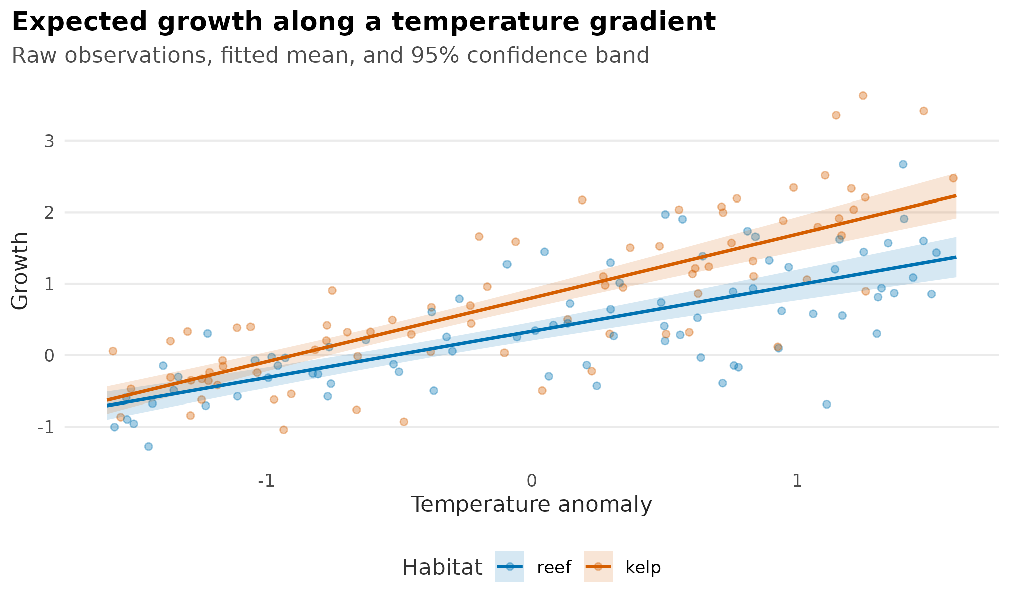
Raw observations and fitted mu surfaces for a Gaussian
location-scale model; ribbons are 95% Wald confidence bands from
predict_parameters().
Distributional-parameter surfaces
The same fit can show more than the mean.
predict_parameters() returns a long table with one row per
distributional parameter, and plot_parameter_surface()
draws estimate lines plus finite interval bands when they are
present.
pred_surface <- rbind(
  pred_mu,
  pred_sigma[pred_sigma$habitat == levels(fish$habitat)[1], , drop = FALSE]
)
pred_surface$surface_group <- as.character(pred_surface$habitat)
pred_surface$surface_group[pred_surface$dpar == "sigma"] <- "shared sigma"
surface_group_palette <- c(
  habitat_palette,
  "shared sigma" = gallery_colour("green")
)

plot_parameter_surface(
  pred_surface,
  x = "temperature",
  colour = "surface_group",
  dpar = c("mu", "sigma"),
  facet = "panel",
  point = FALSE
) +
  scale_colour_manual(
    values = surface_group_palette,
    breaks = c("reef", "kelp", "shared sigma")
  ) +
  scale_fill_manual(
    values = surface_group_palette,
    breaks = c("reef", "kelp", "shared sigma")
  ) +
  labs(
    title = "Mean and residual-scale surfaces",
    subtitle = "Wald bands from predict_parameters(); sigma is shared",
    x = "Temperature anomaly",
    y = "Estimate on response scale",
    colour = NULL
  ) +
  theme_drmtmb_gallery()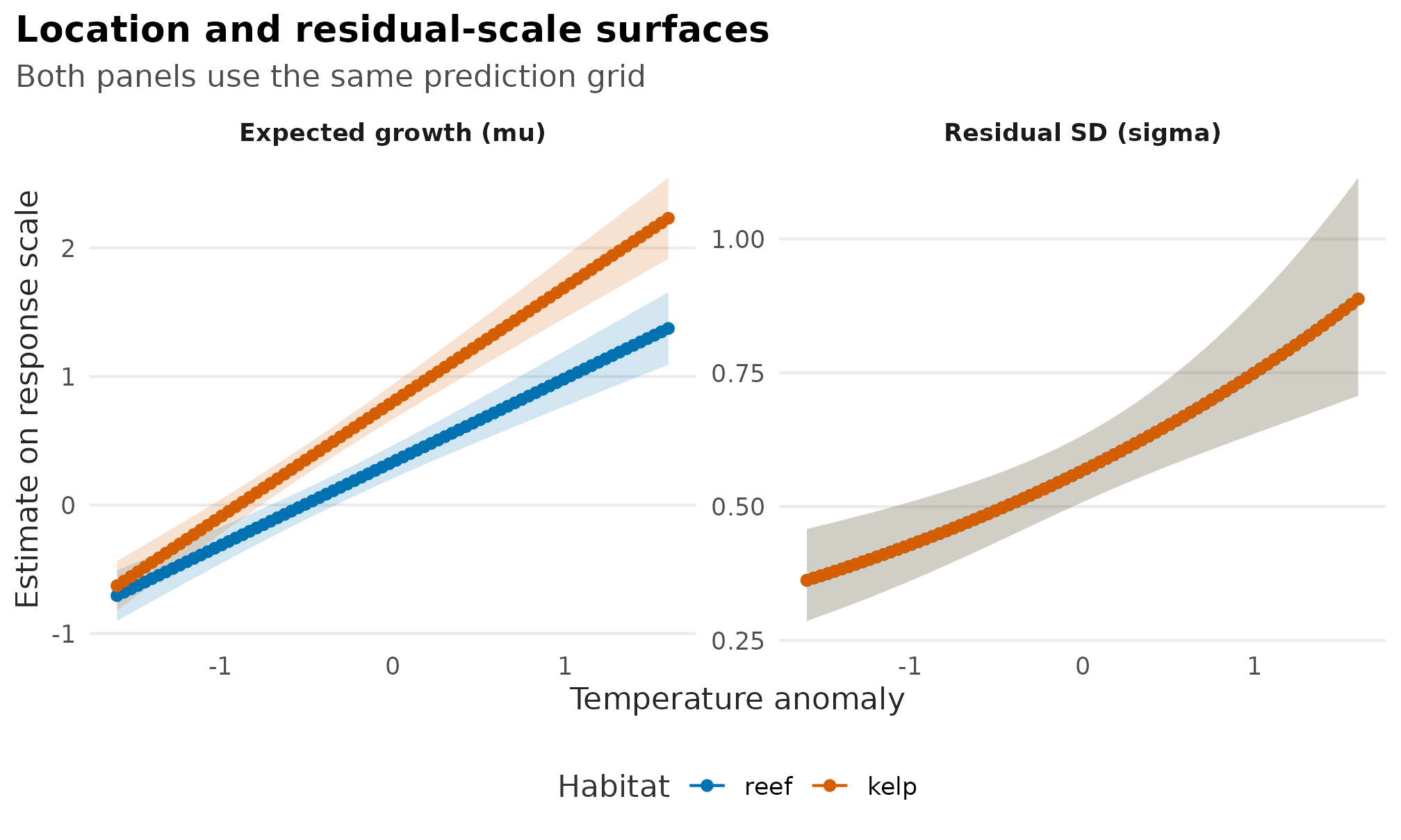
Fitted response-scale mu and sigma surfaces;
ribbons are 95% Wald confidence bands from
predict_parameters(), and sigma is shared
across habitats because the scale formula contains temperature but not
habitat.
The mu panel is the expected response. The
sigma panel is the fitted residual standard deviation, so
an upward line means lower predictability or larger residual
heterogeneity at warmer values.
For scale models, the observed-data analogue is not the raw response
itself. Raw growth lives on the location scale. A useful
scale check is the residual magnitude after subtracting the fitted
mu: under a Gaussian model,
E(|residual|) = sigma * sqrt(2 / pi). This keeps the
observed scatter visible without putting raw response points on a
sigma axis.
pred_row_growth <- predict_parameters(
  fit_growth,
  newdata = fish,
  dpar = c("mu", "sigma")
)
row_mu <- pred_row_growth[pred_row_growth$dpar == "mu", c("row", "estimate")]
row_sigma <- pred_row_growth[
  pred_row_growth$dpar == "sigma",
  c("row", "estimate")
]
names(row_mu)[2] <- "fitted_mu"
names(row_sigma)[2] <- "fitted_sigma"
scale_check <- merge(row_mu, row_sigma, by = "row")
scale_check <- cbind(fish[scale_check$row, ], scale_check)
scale_check$abs_residual <- abs(scale_check$growth - scale_check$fitted_mu)

pred_sigma$expected_abs_residual <- pred_sigma$estimate * sqrt(2 / pi)
pred_sigma$quantity <- "Expected absolute residual"

ggplot(scale_check, aes(temperature, abs_residual, colour = habitat)) +
  geom_point(alpha = 0.22, size = 1.2) +
  geom_line(
    data = pred_sigma,
    aes(
      y = expected_abs_residual,
      colour = quantity,
      group = quantity
    ),
    linewidth = 0.9
  ) +
  scale_colour_manual(values = c(
    habitat_palette,
    "Expected absolute residual" = gallery_colour("green")
  )) +
  labs(
    title = "Residual magnitudes carry the scale information",
    subtitle = "Points are absolute residuals; the green curve is sigma * sqrt(2 / pi)",
    x = "Temperature anomaly",
    y = "Absolute residual",
    colour = NULL
  ) +
  coord_cartesian(ylim = c(0, NA)) +
  theme_drmtmb_gallery()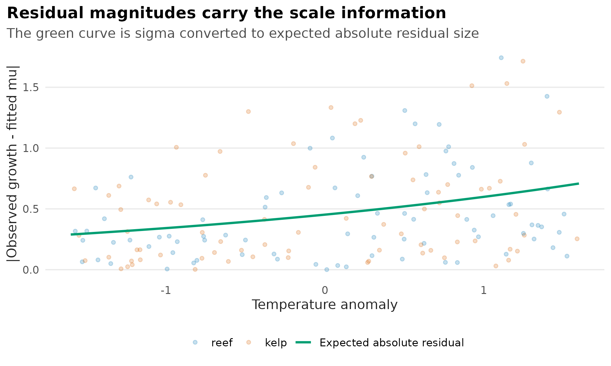
Observed absolute residual magnitudes compared with the fitted
expectation implied by the response-scale sigma surface.
Confidence intervals are only one slice through the uncertainty
surface. This gallery calls the fuller display a Confidence Eye: a pale
confidence region with a hollow point-estimate circle. The idea is close
to Raindrop plots,
but the name and use are deliberately distinct. A Confidence Eye is not
a posterior density; it is a frequentist compatibility display that
gives confidence intervals a visible shape without adding interval bars,
filled estimate dots, or outlines by default. The code below uses a
normal likelihood approximation from the estimate and standard error,
draws the finite 95% confidence region, and keeps the no-effect line and
hollow estimate circle visible together. Both rows are shown on the
fitted coefficient scale so the no-effect line has the same meaning; the
sigma row is a log-SD effect, so positive values mean one
unit of temperature increases residual scale. This shared-axis display
is only appropriate when the predictor scale is common or standardized;
coefficients for different predictors or different units should be
faceted, standardized, or converted to a named contrast before visual
comparison.
coef_growth <- summary(fit_growth)$coefficients
confidence_curves <- rbind(
  make_confidence_eye_distribution(
    parameter = "mu temperature slope",
    estimate = coef_growth["mu:temperature", "estimate"],
    std_error = coef_growth["mu:temperature", "std_error"],
    transform = "identity",
    null_value = 0
  ),
  make_confidence_eye_distribution(
    parameter = "sigma temperature log-SD effect",
    estimate = coef_growth["sigma:temperature", "estimate"],
    std_error = coef_growth["sigma:temperature", "std_error"],
    transform = "identity",
    null_value = 0
  )
)
confidence_curves$parameter <- factor(
  confidence_curves$parameter,
  levels = rev(c("mu temperature slope", "sigma temperature log-SD effect"))
)
confidence_curves$y <- as.numeric(confidence_curves$parameter)
confidence_curves$drop_height <- 0.17 * confidence_curves$height
confidence_reference <- unique(
  confidence_curves[c("parameter", "null_value", "estimate_value")]
)
confidence_reference$y <- as.numeric(confidence_reference$parameter)
confidence_palette <- c(
  "mu temperature slope" = gallery_colour("blue"),
  "sigma temperature log-SD effect" = gallery_colour("green")
)

ggplot(confidence_curves, aes(value, ymin = y - drop_height, ymax = y + drop_height)) +
  geom_ribbon(aes(fill = parameter), alpha = 0.24, colour = NA) +
  geom_vline(
    xintercept = 0,
    linetype = "dotted",
    colour = "grey45",
    linewidth = 0.45
  ) +
  geom_point(
    data = confidence_reference,
    aes(x = estimate_value, y = y, colour = parameter),
    inherit.aes = FALSE,
    shape = 21,
    fill = "white",
    size = 3.1,
    stroke = 1.1
  ) +
  scale_colour_manual(values = confidence_palette) +
  scale_fill_manual(values = confidence_palette) +
  scale_y_continuous(
    breaks = seq_along(levels(confidence_curves$parameter)),
    labels = levels(confidence_curves$parameter),
    expand = expansion(mult = c(0.28, 0.32))
  ) +
  scale_x_continuous(
    breaks = c(0, 0.25, 0.50, 0.75),
    expand = expansion(mult = 0.04)
  ) +
  coord_cartesian(xlim = c(-0.05, 0.82)) +
  labs(
    title = NULL,
    subtitle = NULL,
    x = "Coefficient",
    y = NULL,
    colour = "Parameter"
  ) +
  theme_confidence_eye() +
  theme(
    legend.position = "none"
  )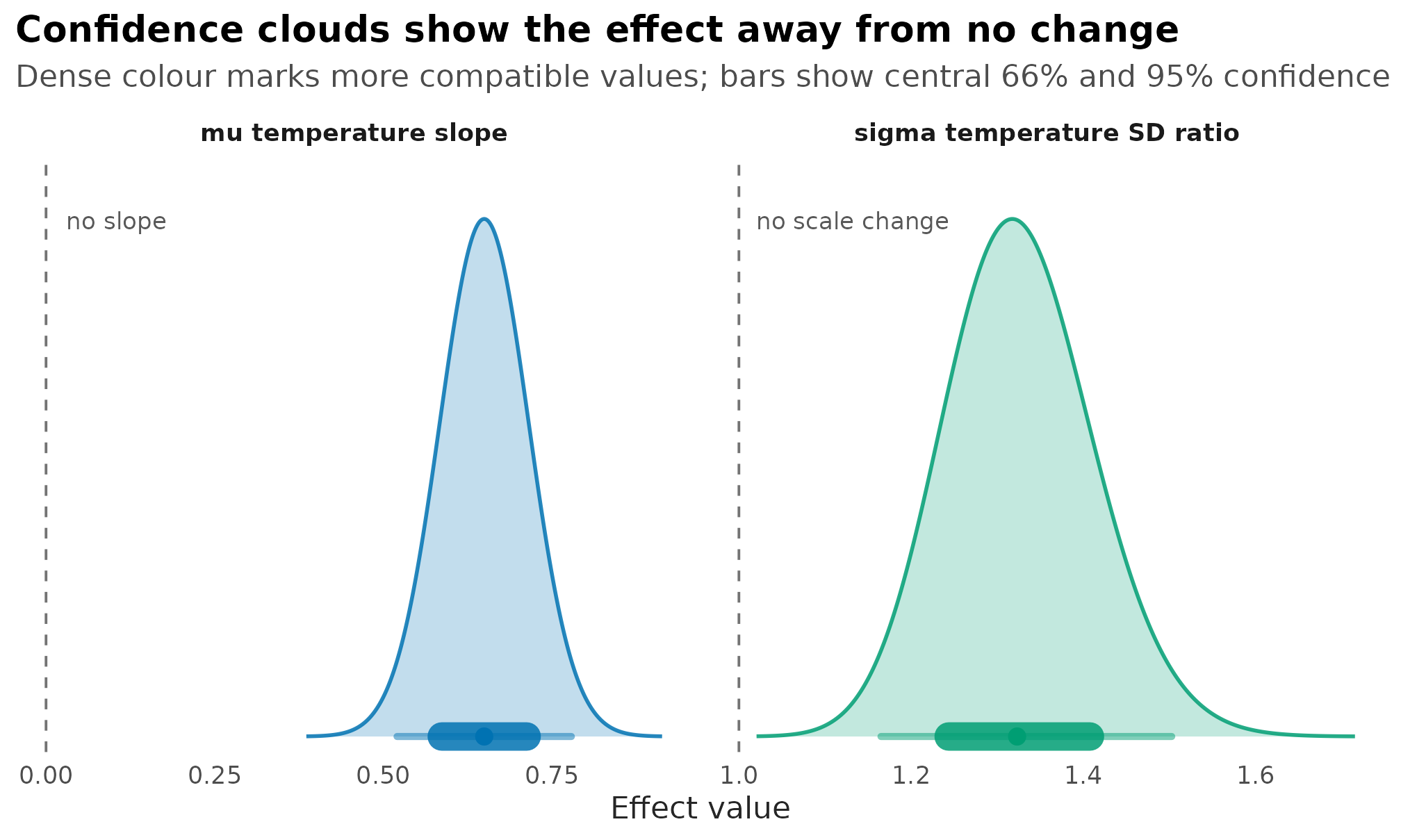
Confidence Eye display for fixed-effect slope estimates; pale regions are finite 95% Wald confidence regions and hollow circles are point estimates.
Distributional parameters are not all residual standard deviations. Shape, inflation, hurdle, and residual-correlation parameters answer different questions and often live on bounded response scales. The next panel set uses three fitted models and the same plotting helper, but each panel names the estimand explicitly.
set.seed(2594)
n_tail <- 2500
tail_dat <- data.frame(tail_pressure = runif(n_tail, -1.5, 1.5))
tail_nu <- 2 + exp(log(4) - tail_dat$tail_pressure)
tail_dat$robust_trait <- 0.35 +
  0.45 * tail_dat$tail_pressure +
  0.55 * stats::rt(n_tail, df = tail_nu)
fit_tail <- drmTMB(
  bf(robust_trait ~ tail_pressure, sigma ~ 1, nu ~ tail_pressure),
  family = student(),
  data = tail_dat
)
tail_grid <- data.frame(tail_pressure = seq(-1.5, 1.5, length.out = 80))
pred_tail <- predict_parameters(
  fit_tail,
  newdata = tail_grid,
  dpar = "nu",
  conf.int = TRUE
)
pred_tail$gradient <- pred_tail$tail_pressure
pred_tail$panel <- "Tail weight (nu)"
pred_tail$model <- "Tail weight"

set.seed(2595)
n_count <- 180
count_dat <- data.frame(detection_difficulty = runif(n_count, -1.2, 1.2))
mu_count <- exp(0.9 + 0.35 * count_dat$detection_difficulty)
zi_count <- plogis(-1.1 + 1.25 * count_dat$detection_difficulty)
count_dat$count <- ifelse(
  runif(n_count) < zi_count,
  0,
  stats::rpois(n_count, mu_count)
)
fit_zi <- drmTMB(
  bf(count ~ detection_difficulty, zi ~ detection_difficulty),
  family = poisson(link = "log"),
  data = count_dat
)
zi_grid <- data.frame(detection_difficulty = seq(-1.2, 1.2, length.out = 80))
pred_zi <- predict_parameters(
  fit_zi,
  newdata = zi_grid,
  dpar = "zi",
  conf.int = TRUE
)
pred_zi$gradient <- pred_zi$detection_difficulty
pred_zi$panel <- "Structural zero (zi)"
pred_zi$model <- "Structural-zero probability"

set.seed(2596)
n_pair <- 160
pair_dat <- data.frame(disturbance = runif(n_pair, -1.4, 1.4))
rho_true <- tanh(-0.15 + 0.75 * pair_dat$disturbance)
z1 <- stats::rnorm(n_pair)
z2 <- stats::rnorm(n_pair)
pair_dat$activity <- 0.25 + 0.35 * pair_dat$disturbance + z1
pair_dat$boldness <- -0.1 +
  0.2 * pair_dat$disturbance +
  rho_true * z1 +
  sqrt(1 - rho_true^2) * z2
fit_pair <- drmTMB(
  bf(
    mu1 = activity ~ disturbance,
    mu2 = boldness ~ disturbance,
    sigma1 ~ 1,
    sigma2 ~ 1,
    rho12 ~ disturbance
  ),
  family = c(gaussian(), gaussian()),
  data = pair_dat
)
rho_grid <- data.frame(disturbance = seq(-1.4, 1.4, length.out = 80))
pred_rho <- predict_parameters(
  fit_pair,
  newdata = rho_grid,
  dpar = "rho12",
  conf.int = TRUE
)
pred_rho$gradient <- pred_rho$disturbance
pred_rho$panel <- "Residual rho12"
pred_rho$model <- "Residual correlation"

common_prediction_columns <- intersect(names(pred_tail), names(pred_zi))

pred_extra <- rbind(
  pred_tail[common_prediction_columns],
  pred_zi[common_prediction_columns],
  pred_rho[common_prediction_columns]
)
pred_extra$panel <- factor(
  pred_extra$panel,
  levels = c(
    "Tail weight (nu)",
    "Structural zero (zi)",
    "Residual rho12"
  )
)

plot_parameter_surface(
  pred_extra,
  x = "gradient",
  colour = "model",
  facet = "panel",
  dpar = c("nu", "zi", "rho12"),
  point = FALSE
) +
  geom_hline(
    data = data.frame(
      .drmTMB_plot_facet = factor(
        "Residual rho12",
        levels = levels(pred_extra$panel)
      )
    ),
    aes(yintercept = 0),
    inherit.aes = FALSE,
    linetype = "dashed",
    colour = "grey55"
  ) +
  scale_colour_manual(values = c(
    "Tail weight" = "#0072B2",
    "Structural-zero probability" = "#009E73",
    "Residual correlation" = "#D55E00"
  )) +
  scale_fill_manual(values = c(
    "Tail weight" = "#0072B2",
    "Structural-zero probability" = "#009E73",
    "Residual correlation" = "#D55E00"
  )) +
  labs(
    title = "Shape, inflation, and residual-correlation panels",
    subtitle = "Each panel is a different distributional parameter on its response scale",
    x = "Predictor gradient",
    y = "Estimate on response scale",
    colour = "Parameter",
    fill = "Parameter"
  ) +
  theme_drmtmb_gallery() +
  theme(legend.position = "none")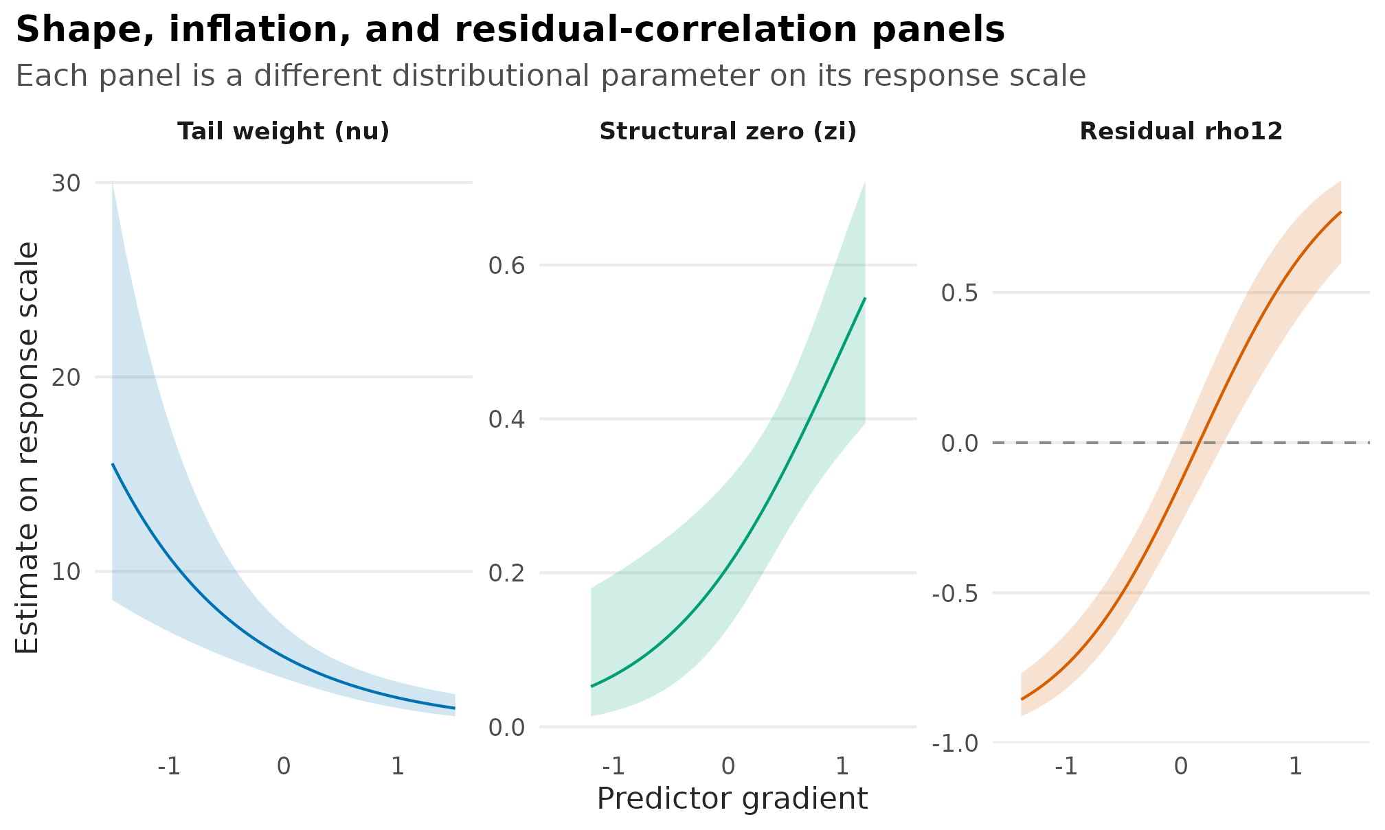
Response-scale distributional-parameter panels for nu,
zi, and residual rho12; ribbons are 95% Wald
confidence bands. The rho12 band is computed for each
supplied newdata row and its coverage is not certified.
The nu panel is a Student-t degrees-of-freedom
parameter: lower values mean heavier tails, and here the fitted model
estimates a changing tail shape through nu ~ tail_pressure.
The zi panel is a structural-zero probability, not a mean
count. The rho12 panel is residual coupling between two
responses after their own means and scales have been modelled.
Distributional adequacy diagnostics
The surfaces above answer “what did the model fit?”. This section
answers the question that should come next: “is that distribution
actually right?” A location-scale model can produce a convincing
mu surface while getting the shape of the residual
distribution wrong, and no amount of looking at fitted means will reveal
it.
worm_plot() and qq_plot() both work from
randomised quantile residuals (Dunn & Smyth, 1996), which are
standard normal under a correctly specified model of any family, so
these diagnostics apply beyond the Gaussian case — see Distributional outputs
and adequacy for the residual definition. A worm plot is a detrended
QQ plot: it draws the deviation of each ordered residual from its
theoretical quantile, a dotted zero reference, and a smoothed trend
through the points. Under an adequate model that trend stays close to
zero, so departures read as shape rather than as a diagonal line. The
plot draws no pointwise envelope, so read the trend qualitatively rather
than as a test.
A diagnostic figure is only informative when the reader can see what
a failure looks like, so this pair uses the same data twice. The first
fit is the correctly specified location-scale model from the previous
section, where sigma ~ temperature matches the
heteroscedastic truth.
wrap_subtitle(worm_plot(fit_growth)) +
  theme_drmtmb_gallery()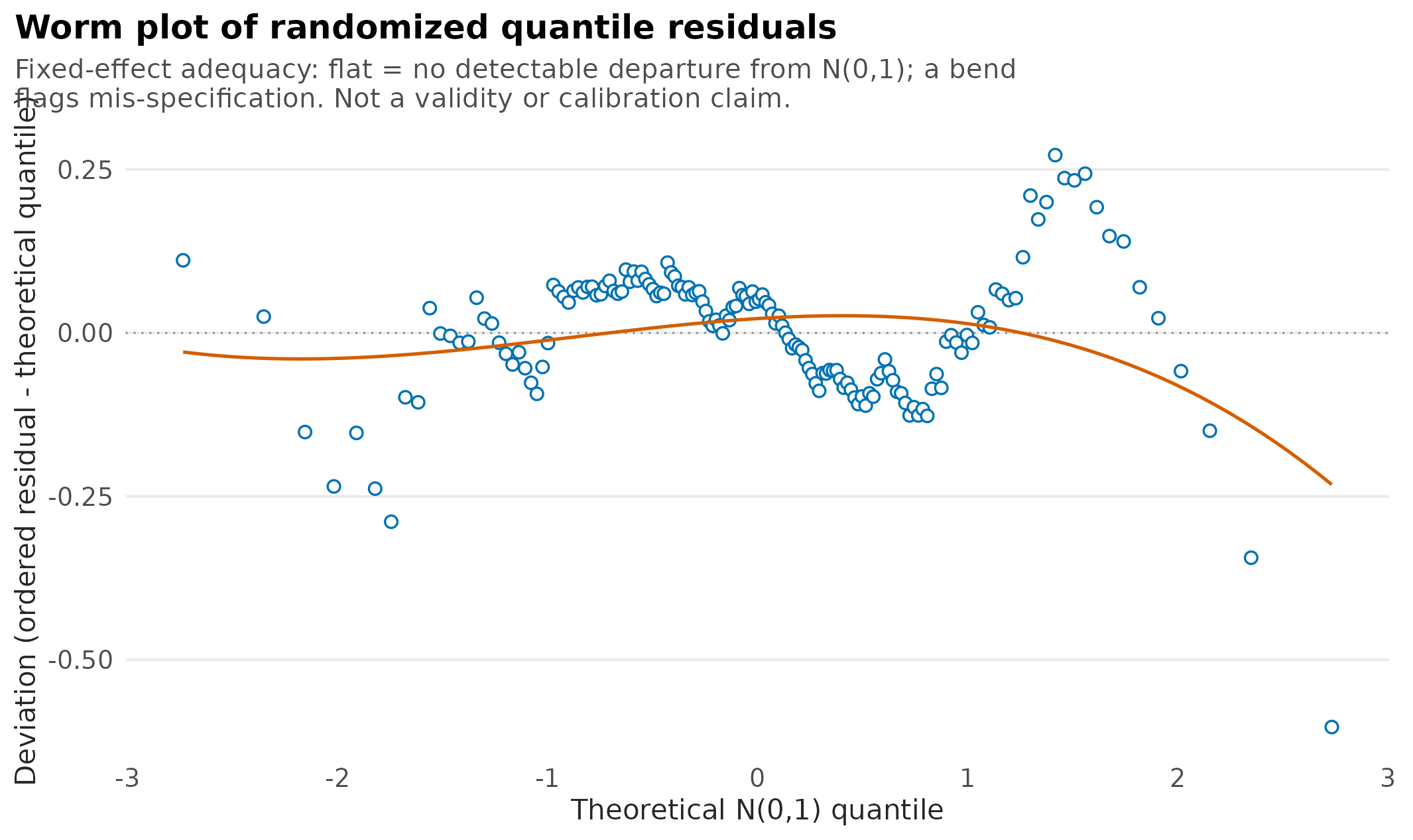
Worm plot of randomised quantile residuals for the correctly specified location-scale model; the smoothed trend holds near the zero reference across the bulk of the distribution, drifting only in the sparse right tail.
The second fit deliberately holds the residual SD constant while the
truth is heteroscedastic. It is the same response, the same predictors,
and the same rows; only the sigma formula changes.
fit_mis <- drmTMB(
  bf(growth ~ temperature * habitat, sigma ~ 1),
  family = gaussian(),
  data = fish
)

wrap_subtitle(worm_plot(fit_mis)) +
  theme_drmtmb_gallery()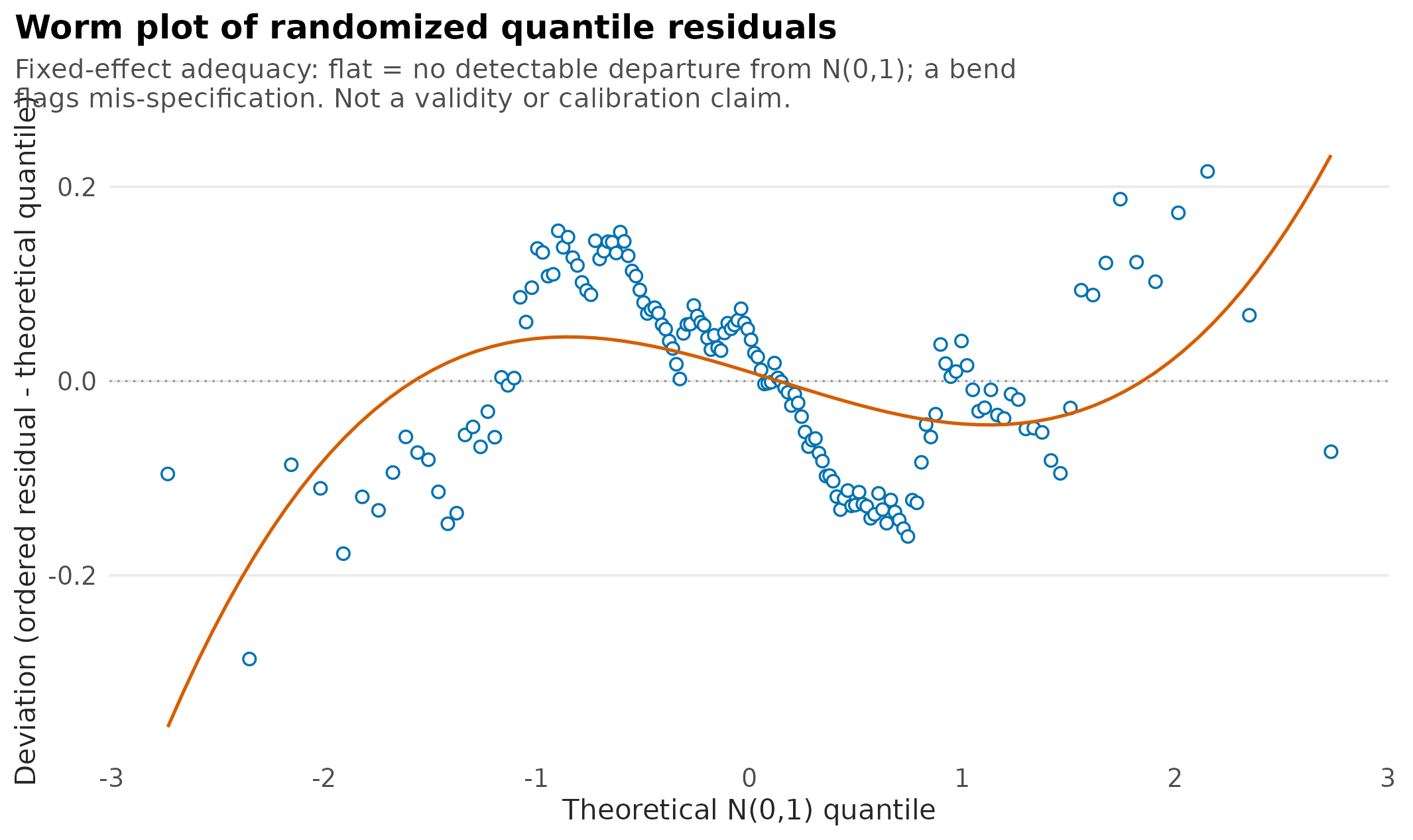
Worm plot for a deliberately mis-specified model that holds
sigma constant while the generating process is
heteroscedastic; the pronounced S-shaped trend is the diagnostic signal.
Read the two together. The scale misfit does not show up as a bad
mean structure, because the mean structure is not what is wrong. It
shows up in the residual shape, which is what the worm plot is built to
expose. This is the practical argument for modelling sigma
rather than assuming it.
Read the bulk, not the extremes. Both panels wander at the far left and right, where a handful of order statistics carry the smoother and it has little to learn from. The adequate model drifts only there; the mis-specified model sweeps a full S across the middle of the distribution, where most of the data sit. A tail excursion in a plot of this size is weak evidence, and neither panel draws an envelope that would tell you how weak.
qq_plot() shows the same residuals without detrending.
It is the more familiar display and the less sensitive one: the same
mild upper-tail departure that the worm plot draws as a downward drift
appears here only as a gentle bow above the identity line, easy to miss
against a straight reference.
wrap_subtitle(qq_plot(fit_growth)) +
  theme_drmtmb_gallery()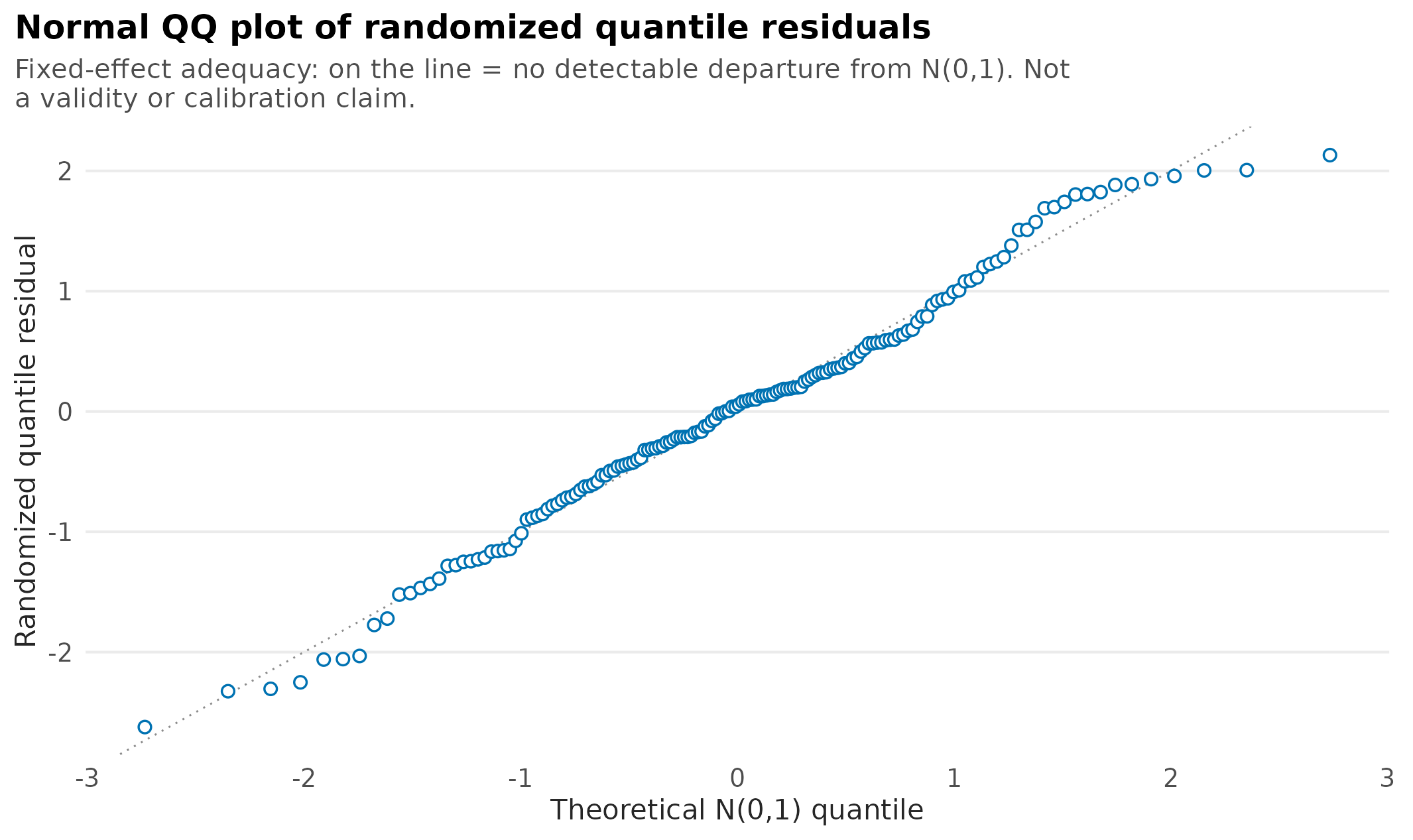
QQ plot of randomised quantile residuals for the correctly specified model; points sit close to the identity reference through the bulk and bow mildly above it in the upper tail. The reference is the identity line, not a fitted line.
centile_chart() answers a different question again.
Rather than asking whether the distribution is adequate, it shows what
the fitted distribution implies for an individual observation:
conditional centiles (percentiles) across a covariate, in the units the
reader measured. For a location-scale model the centiles fan out where
sigma is larger, which is the feature a mean-only model
cannot represent. Read biologically, the plot says an individual fish’s
plausible growth range is wider at high temperature even though the
average trend rises smoothly — the spread, not just the mean, carries
signal.
wrap_subtitle(centile_chart(fit_growth, covariate = "temperature")) +
  scale_colour_viridis_d(option = "viridis", end = 0.9) +
  theme_drmtmb_gallery()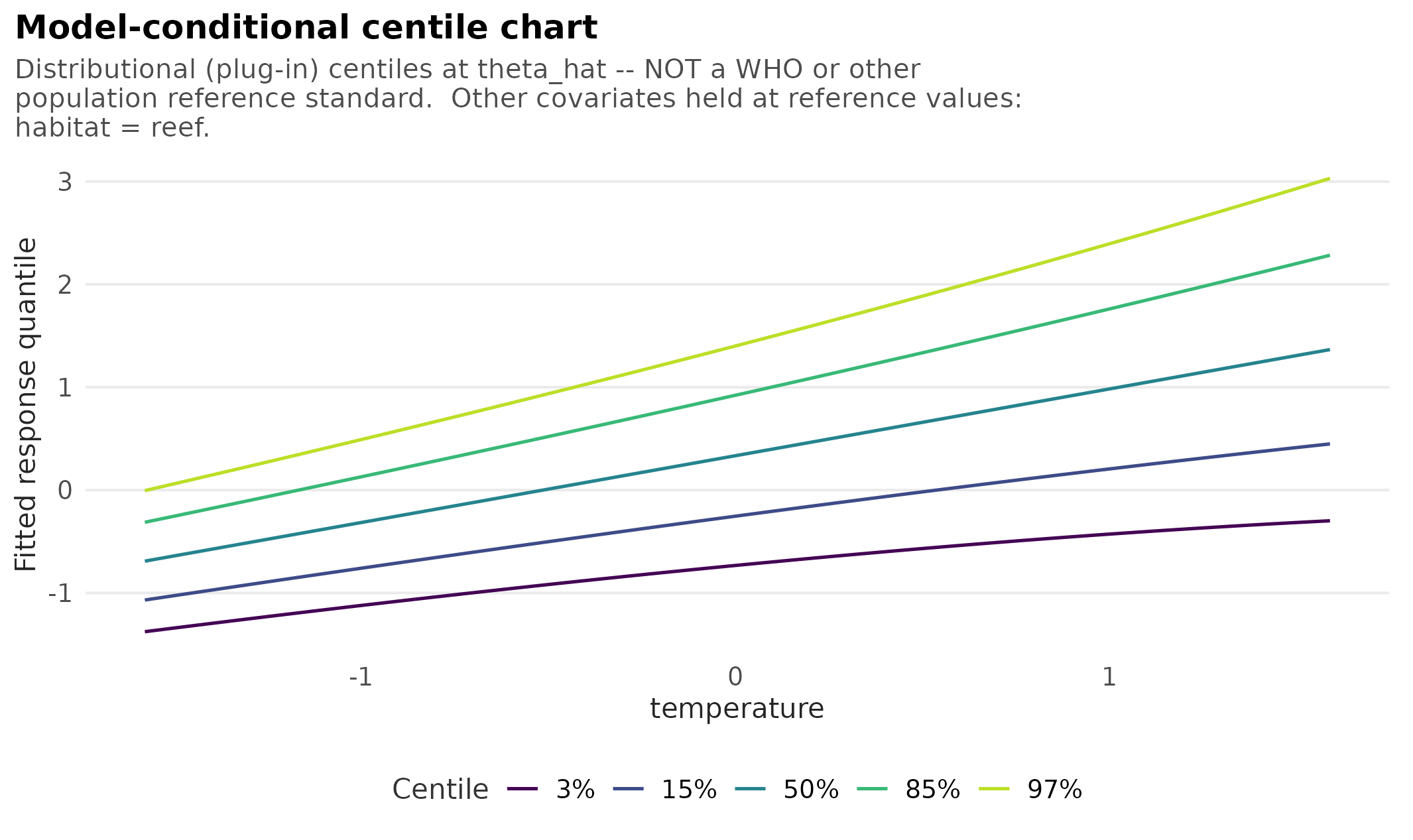
Fitted conditional centiles of growth across temperature; the spread between centiles widens where the fitted residual SD is larger.
Two display choices are worth copying. Centiles are an ordered sequence, so they get an ordered, perceptually uniform palette rather than a categorical one: with a rainbow scale the reader cannot tell from colour alone that 15% lies between 3% and 50%. That palette is also colour-blind-safe, which a red-and-green categorical scale is not.
Centile charts are a distributional-output display, not a diagnostic. They carry no interval for the centile itself: the lines are fitted conditional quantiles, and uncertainty in those quantiles is a separate question this figure does not answer.
Profile-likelihood curves
The Confidence Eye displays earlier in this gallery use Wald intervals, which assume the log-likelihood is quadratic near the estimate. When that assumption is doubtful — small samples, variance and correlation parameters, anything near a boundary — the honest move is to look at the likelihood itself rather than at a quadratic stand-in.
profile() computes the curve and plot()
draws it. First ask the fit which parameters can be profiled and under
what names, because a distributional model has several parameters that
could each be called “the temperature effect”:
head(profile_targets(fit_growth), 8)
#>                               parm target_class  dpar                    term
#> 1             fixef:mu:(Intercept) fixed-effect    mu             (Intercept)
#> 2             fixef:mu:temperature fixed-effect    mu             temperature
#> 3             fixef:mu:habitatkelp fixed-effect    mu             habitatkelp
#> 4 fixef:mu:temperature:habitatkelp fixed-effect    mu temperature:habitatkelp
#> 5          fixef:sigma:(Intercept) fixed-effect sigma             (Intercept)
#> 6          fixef:sigma:temperature fixed-effect sigma             temperature
#>   tmb_parameter index   estimate link_estimate scale   transformation
#> 1       beta_mu     1  0.3342273     0.3342273  link linear_predictor
#> 2       beta_mu     2  0.6497346     0.6497346  link linear_predictor
#> 3       beta_mu     3  0.4669817     0.4669817  link linear_predictor
#> 4       beta_mu     4  0.2440305     0.2440305  link linear_predictor
#> 5    beta_sigma     1 -0.5669660    -0.5669660  link linear_predictor
#> 6    beta_sigma     2  0.2800160     0.2800160  link linear_predictor
#>   target_type profile_ready profile_note
#> 1      direct          TRUE        ready
#> 2      direct          TRUE        ready
#> 3      direct          TRUE        ready
#> 4      direct          TRUE        ready
#> 5      direct          TRUE        ready
#> 6      direct          TRUE        ready
The target strings are explicit, such as
fixef:sigma:temperature. The one below is the temperature
effect on the log residual SD: a scale-side parameter, where the
quadratic Wald assumption is least comfortable.
profile_precision = "fast" coarsens the step controls of
the underlying TMB::tmbprofile() curve; it is fine for a
figure like this, but drop it for a publication interval where the exact
endpoint matters (see Model workflow
for the precision trade-off).
prof_sigma_slope <- profile(
  fit_growth,
  parm = "fixef:sigma:temperature",
  profile_precision = "fast"
)

wrap_subtitle(plot(prof_sigma_slope)) +
  theme_drmtmb_gallery()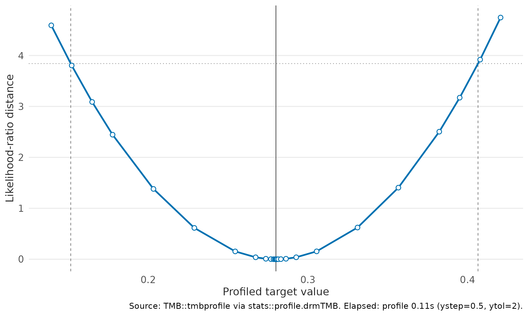
Profile-likelihood curve for the temperature effect on log residual SD, with the 95% profile interval marked; the limits are read from the curve rather than assumed symmetric.
A near-symmetric curve is the reassuring case: it means the Wald interval for that parameter was not misleading. Asymmetry is the finding worth reporting.
Random-effect and variance-component figures
Random-effect figures need a different visual grammar from
residual-scale figures. Residual sigma is the
observation-level standard deviation. A group-level SD, such as the SD
of site intercepts or temperature slopes, is among-group variation in a
fitted random effect.
set.seed(2621)
n_site <- 24
n_site_obs <- 6
site_levels <- seq_len(n_site)
site_random <- data.frame(
  site = factor(site_levels),
  intercept = rnorm(n_site, mean = 0, sd = 0.42),
  slope = rnorm(n_site, mean = 0, sd = 0.24)
)
reef_re <- data.frame(
  site = factor(rep(site_levels, each = n_site_obs), levels = site_levels)
)
reef_re$temperature <- rep(seq(-1, 1, length.out = n_site_obs), n_site)
site_lookup <- as.integer(reef_re$site)
reef_re$growth <- 0.25 +
  0.62 * reef_re$temperature +
  site_random$intercept[site_lookup] +
  site_random$slope[site_lookup] * reef_re$temperature +
  rnorm(nrow(reef_re), mean = 0, sd = 0.34)

fit_re_slopes <- drmTMB(
  bf(growth ~ temperature + (1 + temperature | site), sigma ~ 1),
  family = gaussian(),
  data = reef_re,
  control = drm_control(optimizer = list(eval.max = 160L, iter.max = 160L))
)

component_rows <- summary(fit_re_slopes)$parameters
variance_components <- data.frame(
  component = c(
    "Residual sigma",
    "Site intercept SD",
    "Site temperature-slope SD"
  ),
  component_type = c(
    "Residual scale",
    "Group intercept SD",
    "Group slope SD"
  ),
  estimate = c(
    component_rows["sigma", "estimate"],
    component_rows[
      "sd:mu:(1 + temperature | site):(Intercept)",
      "estimate"
    ],
    component_rows[
      "sd:mu:(1 + temperature | site):temperature",
      "estimate"
    ]
  ),
  response_std_error = c(
    component_rows["sigma", "std_error"],
    component_rows[
      "sd:mu:(1 + temperature | site):(Intercept)",
      "std_error"
    ],
    component_rows[
      "sd:mu:(1 + temperature | site):temperature",
      "std_error"
    ]
  )
)
variance_components$link_estimate <- log(variance_components$estimate)
variance_components$link_std_error <- response_scale_se_to_log_se(
  variance_components$estimate,
  variance_components$response_std_error
)
variance_components <- variance_components[
  is.finite(variance_components$link_std_error),
]
variance_components$component <- factor(
  variance_components$component,
  levels = rev(variance_components$component)
)
variance_components$component_type <- factor(
  variance_components$component_type,
  levels = c("Residual scale", "Group intercept SD", "Group slope SD")
)

component_palette <- c(
  "Residual scale" = gallery_colour("blue"),
  "Group intercept SD" = gallery_colour("green"),
  "Group slope SD" = gallery_colour("orange")
)

component_cloud <- do.call(
  rbind,
  lapply(seq_len(nrow(variance_components)), function(i) {
    row <- variance_components[i, ]
    make_confidence_eye_distribution(
      parameter = row$component,
      estimate = row$link_estimate,
      std_error = row$link_std_error,
      transform = "exp"
    )
  })
)
component_cloud <- merge(
  component_cloud,
  variance_components[c("component", "component_type")],
  by.x = "parameter",
  by.y = "component"
)
component_cloud$parameter <- factor(
  component_cloud$parameter,
  levels = levels(variance_components$component)
)
component_cloud$y_index <- as.numeric(component_cloud$parameter)
component_cloud$ymin <- component_cloud$y_index -
  0.17 * component_cloud$height
component_cloud$ymax <- component_cloud$y_index +
  0.17 * component_cloud$height
variance_components$y_index <- as.numeric(variance_components$component)

ggplot() +
  geom_vline(
    xintercept = 0,
    linetype = "dotted",
    colour = "grey45",
    linewidth = 0.45
  ) +
  geom_ribbon(
    data = component_cloud,
    aes(
      value,
      ymin = ymin,
      ymax = ymax,
      fill = component_type,
      group = parameter
    ),
    alpha = 0.24,
    colour = NA
  ) +
  geom_point(
    data = variance_components,
    aes(estimate, y_index, colour = component_type),
    shape = 21,
    fill = "white",
    size = 3.1,
    stroke = 1.1
  ) +
  scale_colour_manual(values = component_palette) +
  scale_fill_manual(values = component_palette) +
  scale_y_continuous(
    breaks = seq_along(levels(variance_components$component)),
    labels = levels(variance_components$component),
    expand = expansion(add = 0.35)
  ) +
  scale_x_continuous(
    breaks = c(0, 0.1, 0.2, 0.3, 0.4),
    expand = expansion(mult = c(0, 0.04))
  ) +
  coord_cartesian(xlim = c(-0.02, 0.48)) +
  labs(
    title = NULL,
    subtitle = NULL,
    x = "Standard deviation",
    y = NULL,
    colour = "Component"
  ) +
  theme_confidence_eye() +
  guides(colour = "none", fill = "none")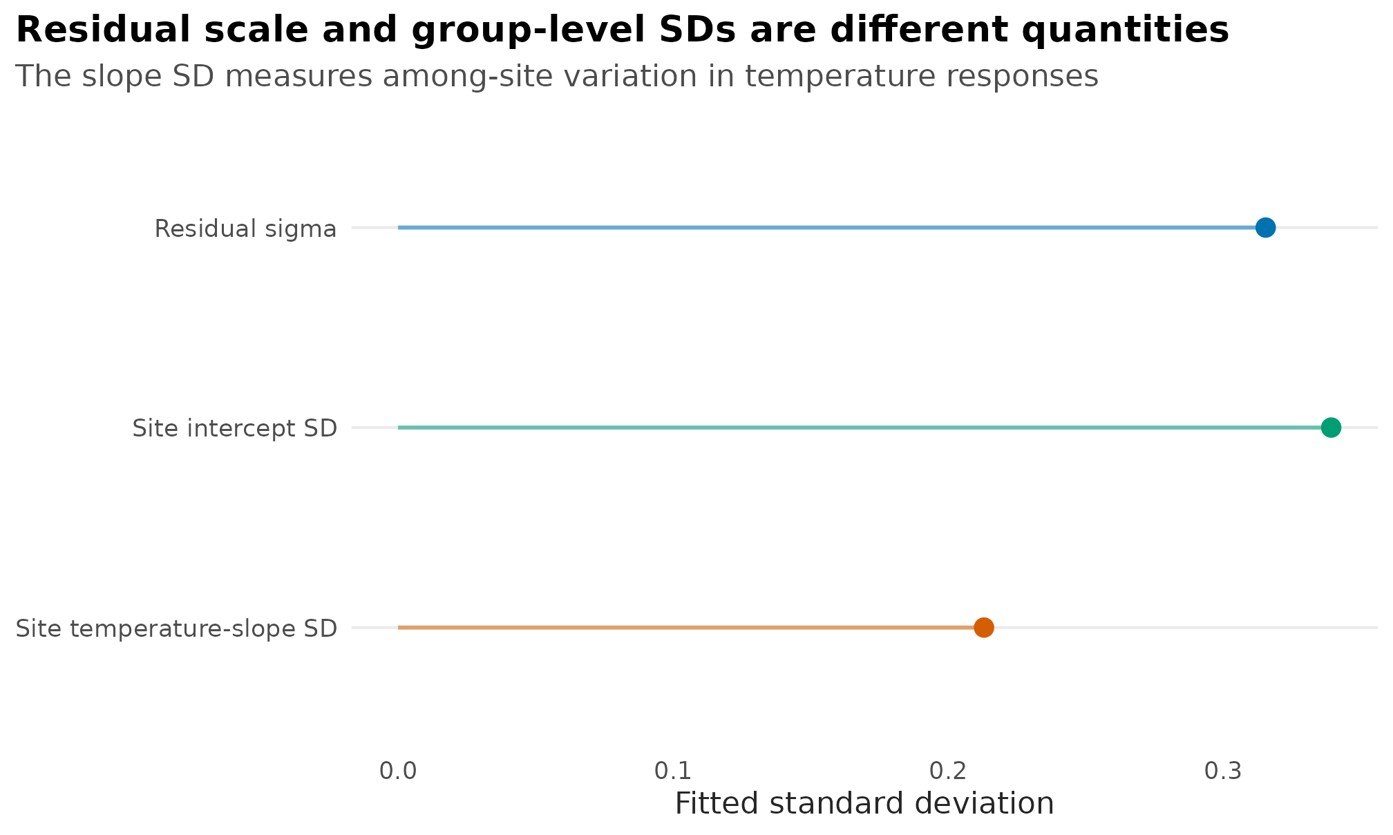
Confidence Eye display for residual and among-site standard deviations; SD intervals are shaped on the fitted log-SD scale and displayed as SDs.
The plot compares three standard deviations, but only one is residual
sigma. The other two are random-effect SDs: how much sites
differ in baseline growth, and how much sites differ in the temperature
slope. The eyes are fast Wald summaries on the log-SD scale. For slower
likelihood-profile intervals on these SDs, use
profile_targets(fit_re_slopes) to choose direct
profile-ready targets rather than profiling every fixed effect by
default.
Readers used to Bayesian model summaries often expect one compact
display that keeps fixed effects, standard deviations, and correlations
together. For this frequentist fit, the Confidence Eye keeps the
confidence region visually subordinate to the estimate: the pale eye is
the finite 95% Wald confidence region and the hollow circle is the point
estimate. This compact panel is a row-by-row reading aid rather than a
magnitude comparison across parameter classes. Fixed effects use their
fitted coefficient scale, SDs are shaped on the log-SD scale and shown
back as SDs, and the correlation is shaped on Fisher’s z
scale and shown back as a correlation.
fixed_rows <- summary(fit_re_slopes)$coefficients
parameter_rows <- summary(fit_re_slopes)$parameters
coefficient_specs <- data.frame(
  group = c(
    "Fixed effects",
    "Fixed effects",
    "SDs (log-scale Wald)",
    "SDs (log-scale Wald)",
    "SDs (log-scale Wald)",
    "Correlation (Fisher-z Wald)"
  ),
  parameter = c(
    "mu intercept",
    "mu temperature slope",
    "residual sigma",
    "site intercept SD",
    "site temperature-slope SD",
    "intercept-slope correlation"
  ),
  display = c(
    "mu\nintercept",
    "mu\ntemperature slope",
    "residual\nsigma",
    "site\nintercept SD",
    "site temperature-\nslope SD",
    "intercept-slope\ncorrelation"
  ),
  estimate = c(
    fixed_rows["mu:(Intercept)", "estimate"],
    fixed_rows["mu:temperature", "estimate"],
    parameter_rows["sigma", "estimate"],
    parameter_rows[
      "sd:mu:(1 + temperature | site):(Intercept)",
      "estimate"
    ],
    parameter_rows[
      "sd:mu:(1 + temperature | site):temperature",
      "estimate"
    ],
    parameter_rows[
      "cor:mu:cor((Intercept),temperature | site)",
      "estimate"
    ]
  ),
  response_std_error = c(
    fixed_rows["mu:(Intercept)", "std_error"],
    fixed_rows["mu:temperature", "std_error"],
    parameter_rows["sigma", "std_error"],
    parameter_rows[
      "sd:mu:(1 + temperature | site):(Intercept)",
      "std_error"
    ],
    parameter_rows[
      "sd:mu:(1 + temperature | site):temperature",
      "std_error"
    ],
    parameter_rows[
      "cor:mu:cor((Intercept),temperature | site)",
      "std_error"
    ]
  ),
  transform = c("identity", "identity", "exp", "exp", "exp", "tanh"),
  reference = c(0, 0, 0, 0, 0, 0),
  stringsAsFactors = FALSE
)
coefficient_specs$link_estimate <- coefficient_specs$estimate
coefficient_specs$link_std_error <- coefficient_specs$response_std_error
sd_rows <- coefficient_specs$transform == "exp"
coefficient_specs$link_estimate[sd_rows] <- log(coefficient_specs$estimate[sd_rows])
coefficient_specs$link_std_error[sd_rows] <- response_scale_se_to_log_se(
  coefficient_specs$estimate[sd_rows],
  coefficient_specs$response_std_error[sd_rows]
)
cor_rows <- coefficient_specs$transform == "tanh"
coefficient_specs$link_estimate[cor_rows] <- atanh(
  guard_rho(coefficient_specs$estimate[cor_rows])
)
coefficient_specs$link_std_error[cor_rows] <- response_scale_se_to_z_se(
  coefficient_specs$estimate[cor_rows],
  coefficient_specs$response_std_error[cor_rows]
)
coefficient_specs <- coefficient_specs[is.finite(coefficient_specs$link_std_error), ]
coefficient_specs$row_id <- rev(seq_len(nrow(coefficient_specs)))
coefficient_specs$group <- factor(
  coefficient_specs$group,
  levels = c(
    "Fixed effects",
    "SDs (log-scale Wald)",
    "Correlation (Fisher-z Wald)"
  )
)
coefficient_cloud <- do.call(
  rbind,
  lapply(seq_len(nrow(coefficient_specs)), function(i) {
    row <- coefficient_specs[i, ]
    make_confidence_eye_distribution(
      parameter = row$parameter,
      estimate = row$link_estimate,
      std_error = row$link_std_error,
      transform = row$transform
    )
  })
)
coefficient_cloud <- merge(
  coefficient_cloud,
  coefficient_specs[c("parameter", "group", "display", "row_id")],
  by = "parameter",
  sort = FALSE
)
coefficient_cloud$group <- factor(
  coefficient_cloud$group,
  levels = levels(coefficient_specs$group)
)
coefficient_cloud$ymin <- coefficient_cloud$row_id -
  0.17 * coefficient_cloud$height
coefficient_cloud$ymax <- coefficient_cloud$row_id +
  0.17 * coefficient_cloud$height

interval_group_palette <- c(
  "Fixed effects" = gallery_colour("blue"),
  "SDs (log-scale Wald)" = gallery_colour("green"),
  "Correlation (Fisher-z Wald)" = gallery_colour("orange")
)

ggplot() +
  geom_vline(
    xintercept = seq(-0.5, 0.75, by = 0.25),
    colour = "grey90",
    linewidth = 0.35
  ) +
  geom_vline(
    xintercept = 0,
    linetype = "dotted",
    colour = "grey55",
    linewidth = 0.55
  ) +
  geom_ribbon(
    data = coefficient_cloud,
    aes(x = value, ymin = ymin, ymax = ymax, fill = group, group = parameter),
    alpha = 0.24,
    colour = NA
  ) +
  geom_point(
    data = coefficient_specs,
    aes(x = estimate, y = row_id, colour = group),
    shape = 21,
    fill = "white",
    size = 3.1,
    stroke = 1.1
  ) +
  scale_colour_manual(values = interval_group_palette) +
  scale_fill_manual(values = interval_group_palette) +
  scale_x_continuous(
    limits = c(-0.5, 0.75),
    breaks = c(-0.5, 0, 0.5),
    expand = expansion(mult = 0.04)
  ) +
  scale_y_continuous(
    breaks = coefficient_specs$row_id,
    labels = coefficient_specs$display,
    expand = expansion(add = 0.42)
  ) +
  labs(
    title = NULL,
    subtitle = NULL,
    x = "Estimate",
    y = NULL,
    colour = NULL
  ) +
  theme_drmtmb_gallery() +
  theme(
    axis.text.y = element_text(size = 10.5, colour = "grey30"),
    axis.ticks.y = element_blank(),
    axis.line.x = element_line(colour = "grey35", linewidth = 0.35),
    axis.ticks.x = element_line(colour = "grey35", linewidth = 0.35),
    axis.ticks.length.x = grid::unit(3, "pt"),
    panel.grid = element_blank()
  ) +
  guides(colour = "none", fill = "none")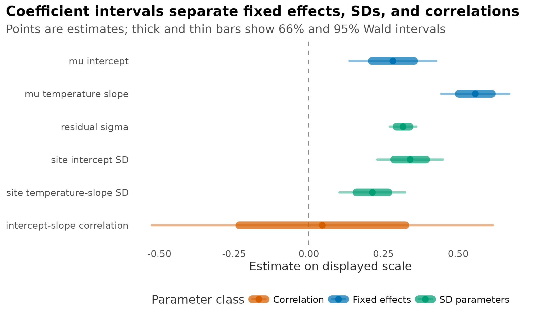
Mixed-parameter Confidence Eye display; fixed effects use fitted-scale Wald intervals, SD rows use log-SD shaping, and the correlation row uses Fisher-z shaping.
A random-slope figure should show repeated site behaviour. The translucent lines below are conditional site-level trajectories: each site borrows strength from the population fit, but sites can still differ in both intercept and temperature slope.
site_intercept <- ranef(fit_re_slopes, "mu")$terms[[
  "(1 + temperature | site):(Intercept)"
]]
site_slope_deviation <- ranef(fit_re_slopes, "mu")$terms[[
  "(1 + temperature | site):temperature"
]]
site_effects <- data.frame(
  site = names(site_slope_deviation),
  intercept_deviation = unname(site_intercept),
  slope_deviation = unname(site_slope_deviation)
)
site_effects$slope_direction <- factor(
  ifelse(
    site_effects$slope_deviation < 0,
    "Lower than average",
    "Higher than average"
  ),
  levels = c("Lower than average", "Higher than average")
)
fixed_re <- summary(fit_re_slopes)$coefficients
site_lines <- expand.grid(
  site = names(site_slope_deviation),
  temperature = seq(-1, 1, length.out = 50),
  KEEP.OUT.ATTRS = FALSE
)
site_lines <- merge(site_lines, site_effects, by = "site")
site_lines$fitted_growth <- (
  fixed_re["mu:(Intercept)", "estimate"] +
    site_lines$intercept_deviation
) + (
  fixed_re["mu:temperature", "estimate"] +
    site_lines$slope_deviation
) * site_lines$temperature
population_line <- data.frame(
  temperature = seq(-1, 1, length.out = 80)
)
population_line$fitted_growth <- fixed_re["mu:(Intercept)", "estimate"] +
  fixed_re["mu:temperature", "estimate"] * population_line$temperature

ggplot() +
  geom_point(
    data = reef_re,
    aes(temperature, growth),
    colour = "grey55",
    alpha = 0.38,
    size = 1.15
  ) +
  geom_line(
    data = site_lines,
    aes(
      temperature,
      fitted_growth,
      group = site,
      colour = slope_direction
    ),
    alpha = 0.48,
    linewidth = 0.55
  ) +
  geom_line(
    data = population_line,
    aes(temperature, fitted_growth),
    colour = gallery_colour("charcoal"),
    linewidth = 1.05
  ) +
  scale_colour_manual(values = c(
    "Lower than average" = gallery_colour("blue"),
    "Higher than average" = gallery_colour("orange")
  )) +
  labs(
    title = "Site trajectories show random slopes",
    subtitle = "Lines are conditional modes, not interval uncertainty",
    x = "Temperature anomaly",
    y = "Growth",
    colour = "Site slope"
  ) +
  theme_drmtmb_gallery()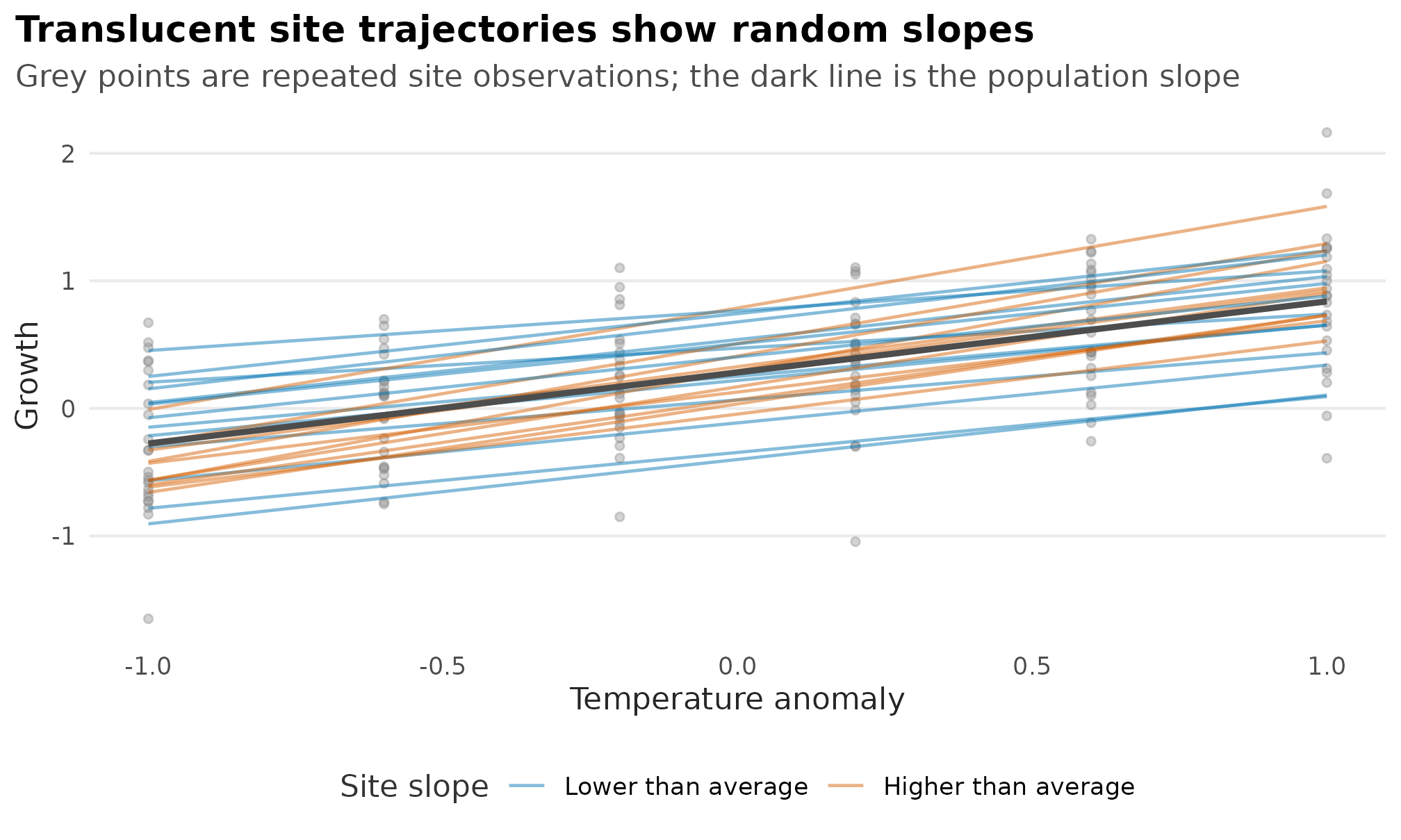
Repeated-measures raw observations with conditional site trajectories and the population-average fitted trend; the figure shows fitted modes, not interval uncertainty.
A direct sd(site) ~ reef_cover formula asks a third
question: does a site-level predictor change the among-site SD in
expected growth? The prediction table keeps this target as
sd(site), not residual sigma.
set.seed(2622)
n_sd_site <- 28
n_sd_each <- 5
site_sd_data <- data.frame(
  site = factor(seq_len(n_sd_site)),
  reef_cover = runif(n_sd_site, -1.2, 1.2)
)
site_sd <- exp(-0.6 + 0.45 * site_sd_data$reef_cover)
site_deviation <- rnorm(n_sd_site, mean = 0, sd = site_sd)
reef_sd <- site_sd_data[rep(seq_len(n_sd_site), each = n_sd_each), ]
reef_sd$temperature <- rep(seq(-1.2, 1.2, length.out = n_sd_each), n_sd_site)
reef_sd$growth <- 0.4 +
  0.5 * reef_sd$temperature +
  site_deviation[as.integer(reef_sd$site)] +
  rnorm(nrow(reef_sd), mean = 0, sd = 0.35)

fit_site_sd <- drmTMB(
  bf(growth ~ temperature + (1 | site), sigma ~ 1, sd(site) ~ reef_cover),
  family = gaussian(),
  data = reef_sd,
  control = drm_control(optimizer = list(eval.max = 180L, iter.max = 180L))
)

grid_site_sd <- prediction_grid(
  fit_site_sd,
  focal = "reef_cover",
  at = list(reef_cover = seq(-1.2, 1.2, length.out = 80))
)
pred_site_sd <- predict_parameters(
  fit_site_sd,
  newdata = grid_site_sd,
  dpar = "sd(site)",
  conf.int = TRUE
)
pred_site_sd$quantity <- "Among-site SD"

plot_parameter_surface(
  pred_site_sd,
  x = "reef_cover",
  colour = "quantity",
  facet = NULL,
  point = FALSE
) +
  scale_colour_manual(values = c(
    "Among-site SD" = gallery_colour("green")
  )) +
  geom_rug(
    data = site_sd_data,
    aes(x = reef_cover),
    inherit.aes = FALSE,
    sides = "b",
    colour = "grey55",
    alpha = 0.50,
    linewidth = 0.45
  ) +
  geom_point(
    data = pred_site_sd[seq(1, nrow(pred_site_sd), length.out = 9), ],
    aes(reef_cover, estimate),
    inherit.aes = FALSE,
    colour = gallery_colour("green"),
    fill = "white",
    shape = 21,
    size = 1.7,
    stroke = 0.55
  ) +
  labs(
    title = "Fitted among-site SD surface",
    subtitle = "Rug marks support; profile/bootstrap intervals needed",
    x = "Reef cover",
    y = "Estimated among-site SD",
    colour = NULL
  ) +
  theme_drmtmb_gallery() +
  guides(colour = "none")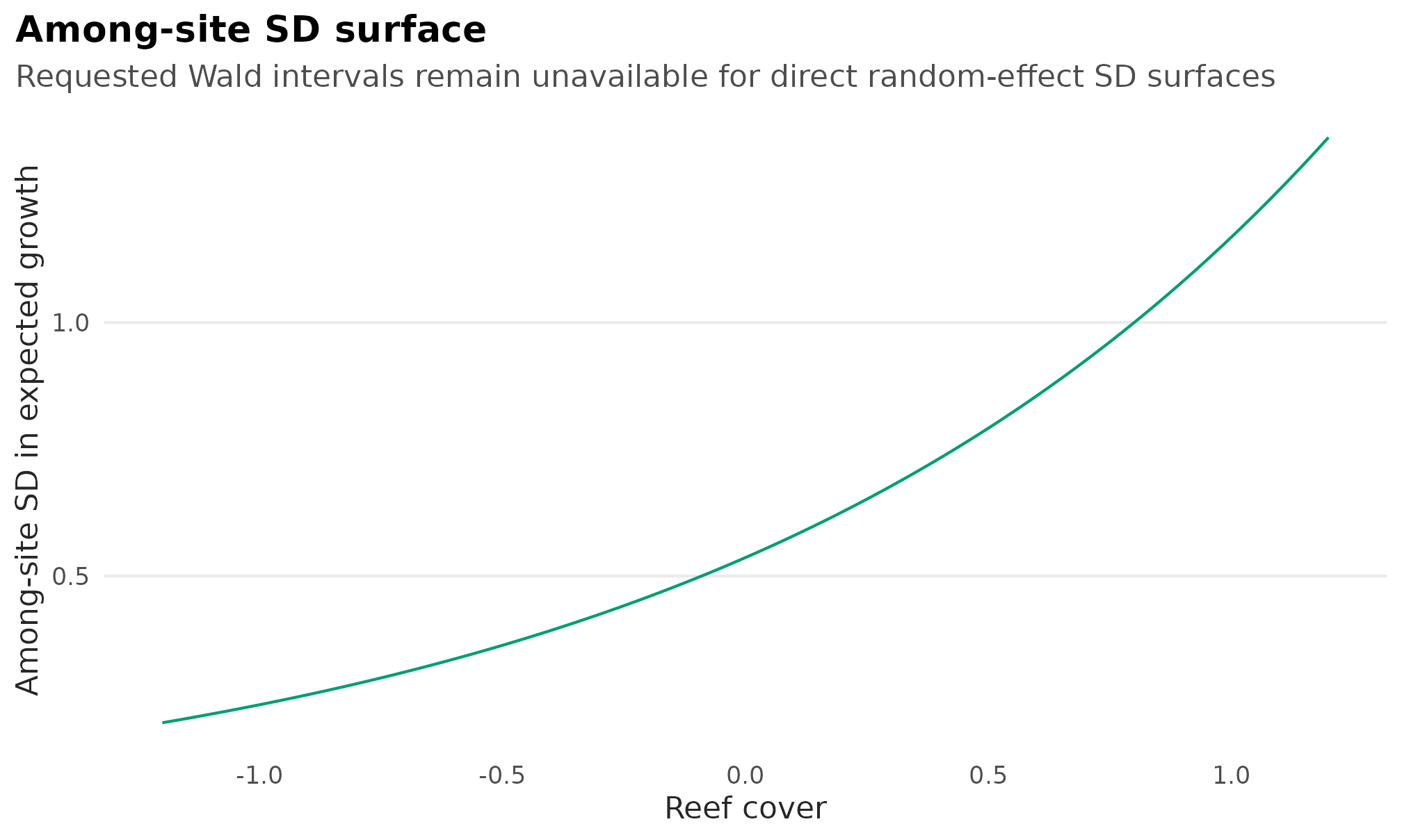
Fitted among-site random-intercept SD surface along reef cover; the rug
shows site-level support, and no band is drawn because the table reports
conf.status = "wald_unavailable" for this derived surface.
This line is a fitted random-effect SD surface. It should not be read
as a raw growth curve, and it should not be overlaid with raw
growth points. The grey rug marks show where the site-level
predictor was observed. The table behind the plot reports
conf.status = "wald_unavailable", which is the honest
interval boundary until a profile or bootstrap route is attached to
these derived surfaces.
Discrete comparisons
For a factor predictor, the same plotting helper uses interval bars rather than ribbons. This is useful for compact tutorial figures and estimated marginal comparisons.
habitat_grid <- data.frame(
  temperature = 0,
  habitat = factor(c("reef", "kelp"), levels = levels(fish$habitat))
)
pred_habitat <- predict_parameters(
  fit_growth,
  newdata = habitat_grid,
  dpar = "mu",
  conf.int = TRUE
)

ggplot(pred_habitat, aes(estimate, habitat, colour = habitat)
) +
  geom_segment(
    aes(x = conf.low, xend = conf.high, yend = habitat),
    linewidth = 0.75,
    lineend = "round"
  ) +
  geom_point(size = 2.7) +
  scale_drmtmb_colour +
  scale_x_continuous(expand = expansion(mult = c(0.04, 0.08))) +
  labs(
    title = "Fitted habitat means at average temperature",
    subtitle = "Intervals are Wald intervals from predict_parameters()",
    x = "Expected growth",
    y = NULL,
    colour = NULL
  ) +
  theme_point_interval_gallery() +
  guides(colour = "none")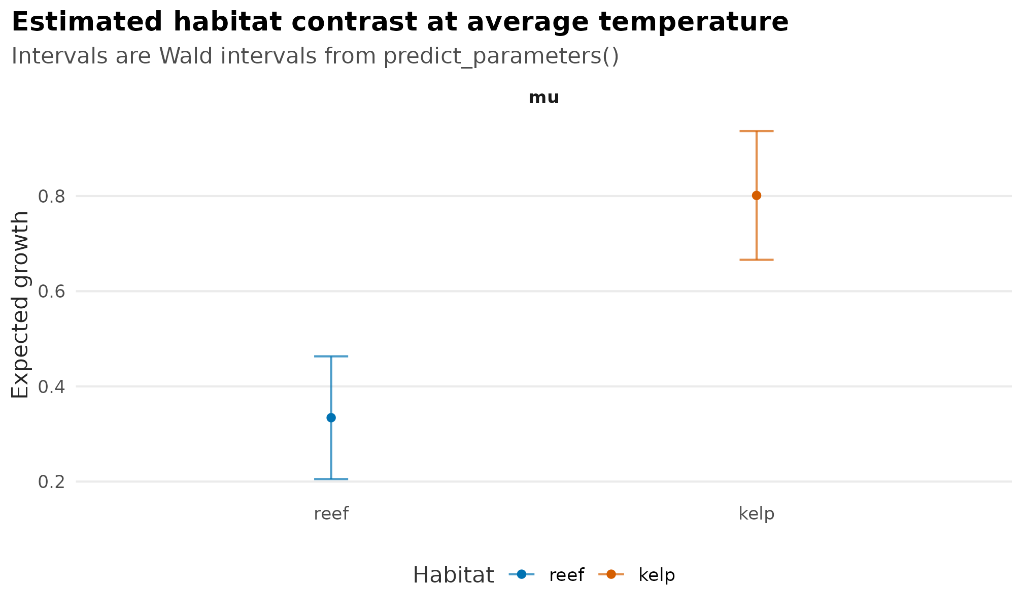
Fitted habitat means at average temperature; points and horizontal
intervals are response-scale Wald summaries from
predict_parameters().
Categorical by categorical interaction
For two categorical predictors, show every fitted cell and its interval. Use position dodging so the uncertainty intervals do not sit on top of each other. Raw observations can sit behind the intervals when they help readers see the data support for each cell.
set.seed(2592)
n_cell <- 30
reef <- expand.grid(
  habitat = factor(habitat_levels, levels = habitat_levels),
  season = factor(c("dry", "wet"), levels = c("dry", "wet")),
  replicate = seq_len(n_cell)
)
reef$mu <- with(
  reef,
  0.6 +
    0.35 * (habitat == "kelp") -
    0.15 * (season == "wet") +
    0.45 * (habitat == "kelp") * (season == "wet")
)
reef$growth <- rnorm(nrow(reef), mean = reef$mu, sd = 0.45)

fit_cat_cat <- drmTMB(
  bf(growth ~ habitat * season, sigma ~ 1),
  family = gaussian(),
  data = reef
)

grid_cat_cat <- expand.grid(
  habitat = levels(reef$habitat),
  season = levels(reef$season)
)
pred_cat_cat <- predict_parameters(
  fit_cat_cat,
  newdata = grid_cat_cat,
  dpar = "mu",
  conf.int = TRUE
)

raw_cat_cat <- reef

cat_cat_position <- position_dodge(width = 0.45)

ggplot(pred_cat_cat, aes(habitat, estimate, colour = season)) +
  geom_point(
    data = raw_cat_cat,
    aes(y = growth, colour = season),
    position = position_jitterdodge(
      jitter.width = 0.08,
      jitter.height = 0,
      dodge.width = 0.45
    ),
    alpha = 0.22,
    size = 1.1,
    show.legend = FALSE
  ) +
  geom_errorbar(
    aes(ymin = conf.low, ymax = conf.high),
    position = cat_cat_position,
    width = 0.08,
    linewidth = 0.65
  ) +
  geom_point(
    position = cat_cat_position,
    size = 2.3
  ) +
  scale_colour_manual(values = season_palette) +
  labs(
    title = "Habitat-season fitted means",
    subtitle = "Small points are observations; large points and bars are fitted mu summaries",
    x = "Habitat",
    y = "Growth",
    colour = "Season"
  ) +
  theme_drmtmb_gallery()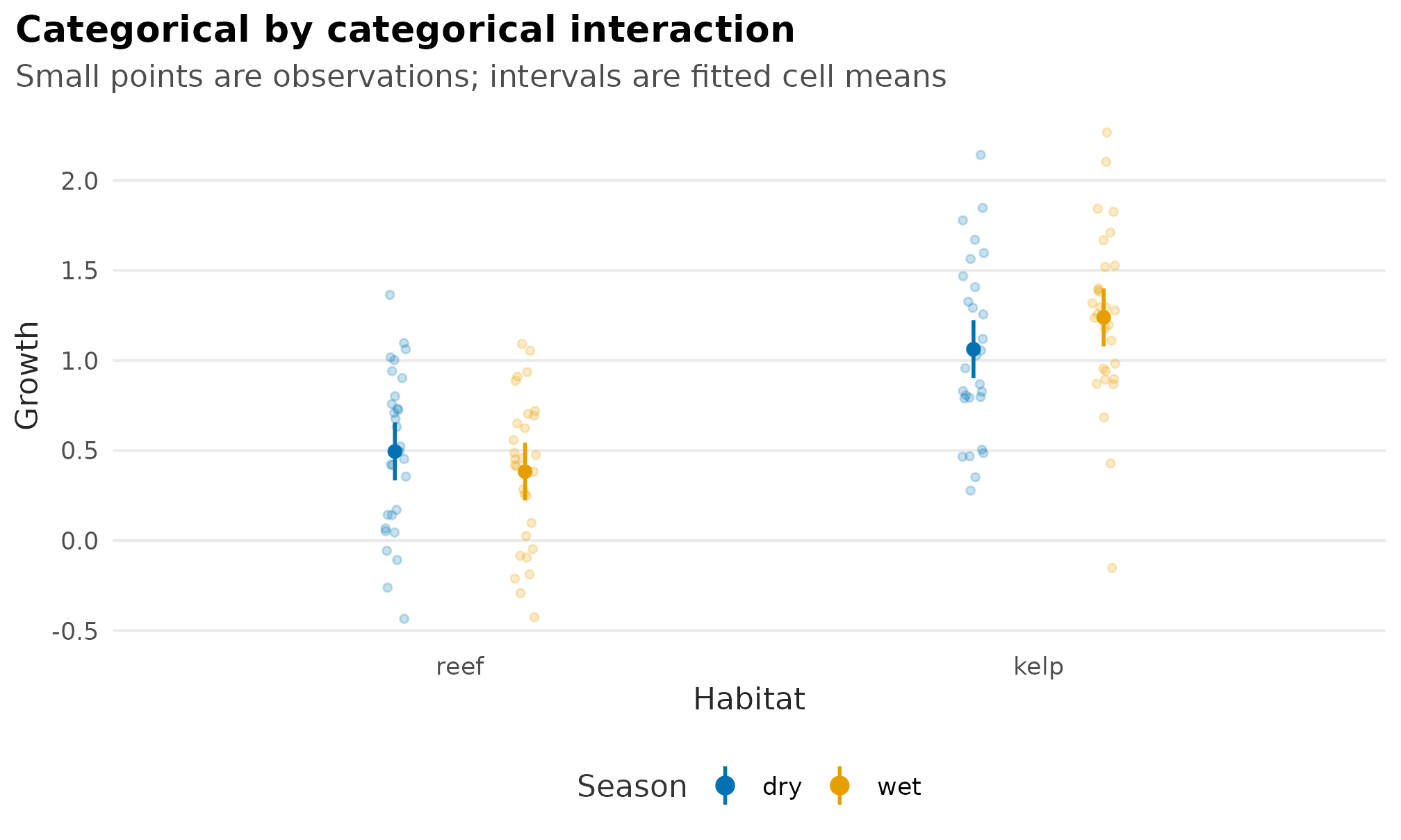
Habitat-by-season fitted mean summaries over raw observations; large
points are fitted mu cell means and bars are 95% Wald
intervals.
Estimated marginal means and marginal summaries
For the first supported emmeans path, a fixed-effect
univariate mu model can produce estimated marginal means
that are easy to turn into publication-style figures. The same rule
applies: keep the target and conditioning values visible. These displays
are mu summaries, not sigma, fitted-response,
random-effect, or bivariate summaries.
emm_habitat <- suppressMessages(
  as.data.frame(
    emmeans::emmeans(
      fit_growth,
      ~ habitat,
      at = list(temperature = 0),
      type = "response"
    )
  )
)

ggplot(emm_habitat, aes(emmean, habitat, colour = habitat)) +
  geom_segment(
    aes(x = asymp.LCL, xend = asymp.UCL, yend = habitat),
    linewidth = 0.75,
    lineend = "round"
  ) +
  geom_point(size = 2.7) +
  scale_drmtmb_colour +
  scale_x_continuous(expand = expansion(mult = c(0.04, 0.08))) +
  labs(
    title = "Estimated marginal means from emmeans",
    subtitle = "Supported fixed-effect mu target, conditioned at temperature = 0",
    x = "Expected growth",
    y = NULL,
    colour = NULL
  ) +
  theme_point_interval_gallery() +
  guides(colour = "none")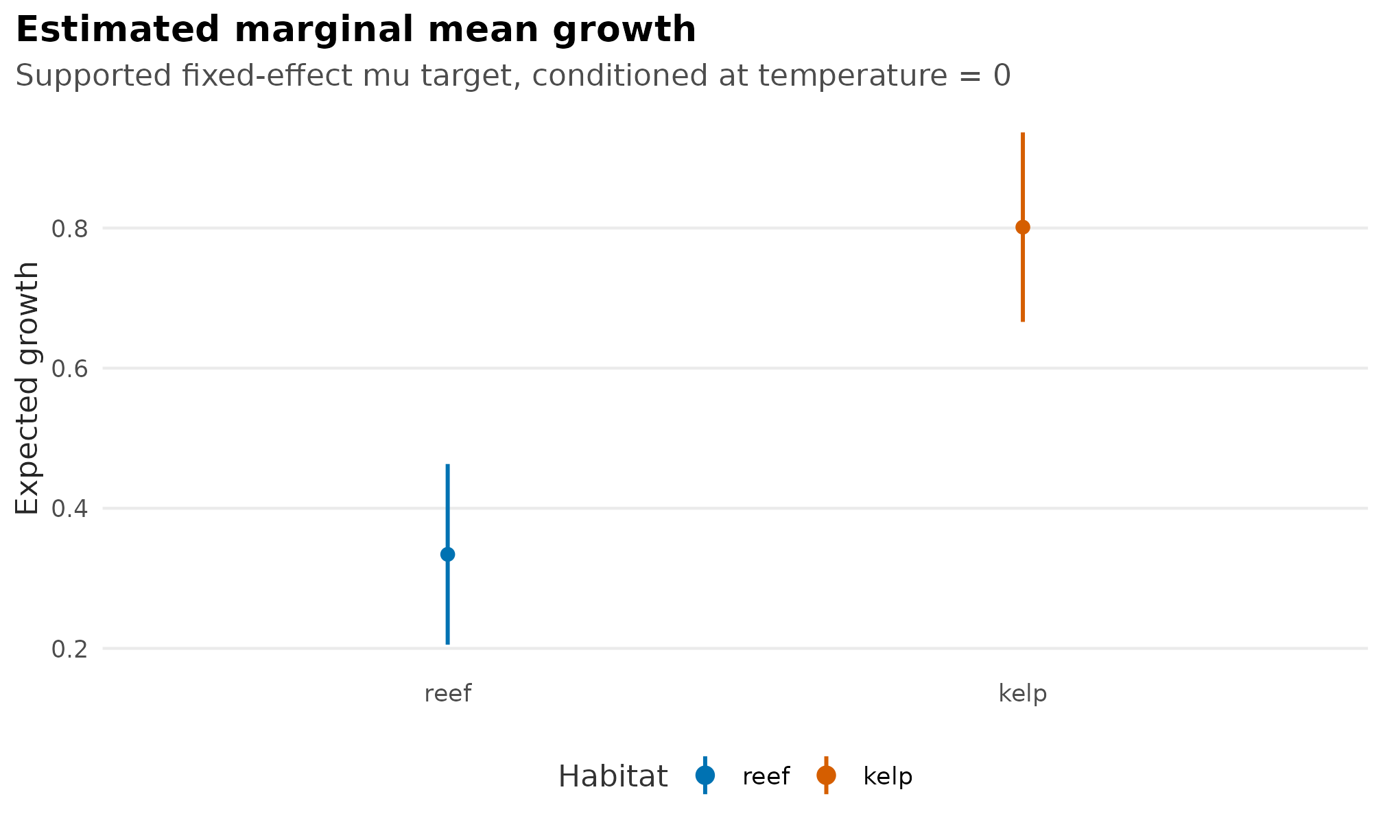
Estimated marginal mean mu summaries for habitat at
temperature zero, using the emmeans bridge for fixed-effect
univariate means.
emmeans reference grids can also condition on a factor.
In the next display, the mu cell means are grouped by
season, so the reader sees the fitted habitat contrast inside each
season rather than a single averaged contrast.
emm_season <- suppressMessages(
  as.data.frame(
    emmeans::emmeans(
      fit_cat_cat,
      ~ habitat | season,
      type = "response"
    )
  )
)
emm_season$habitat_index <- as.numeric(emm_season$habitat)
emm_season$season_offset <- ifelse(emm_season$season == "dry", -0.08, 0.08)
emm_season$habitat_y <- emm_season$habitat_index + emm_season$season_offset

ggplot(emm_season, aes(emmean, habitat_y, colour = season)) +
  geom_segment(
    aes(x = asymp.LCL, xend = asymp.UCL, yend = habitat_y),
    linewidth = 0.7,
    lineend = "round"
  ) +
  geom_point(size = 2.6) +
  scale_colour_manual(values = season_palette) +
  scale_x_continuous(expand = expansion(mult = c(0.05, 0.08))) +
  scale_y_continuous(
    breaks = seq_along(levels(emm_season$habitat)),
    labels = levels(emm_season$habitat),
    limits = c(0.65, length(levels(emm_season$habitat)) + 0.35)
  ) +
  labs(
    title = "Season-conditioned marginal means",
    subtitle = "Habitat mu summaries are shown separately for each season",
    x = "Expected growth",
    y = "Habitat",
    colour = "Season"
  ) +
  theme_point_interval_gallery() +
  theme(legend.position = "bottom")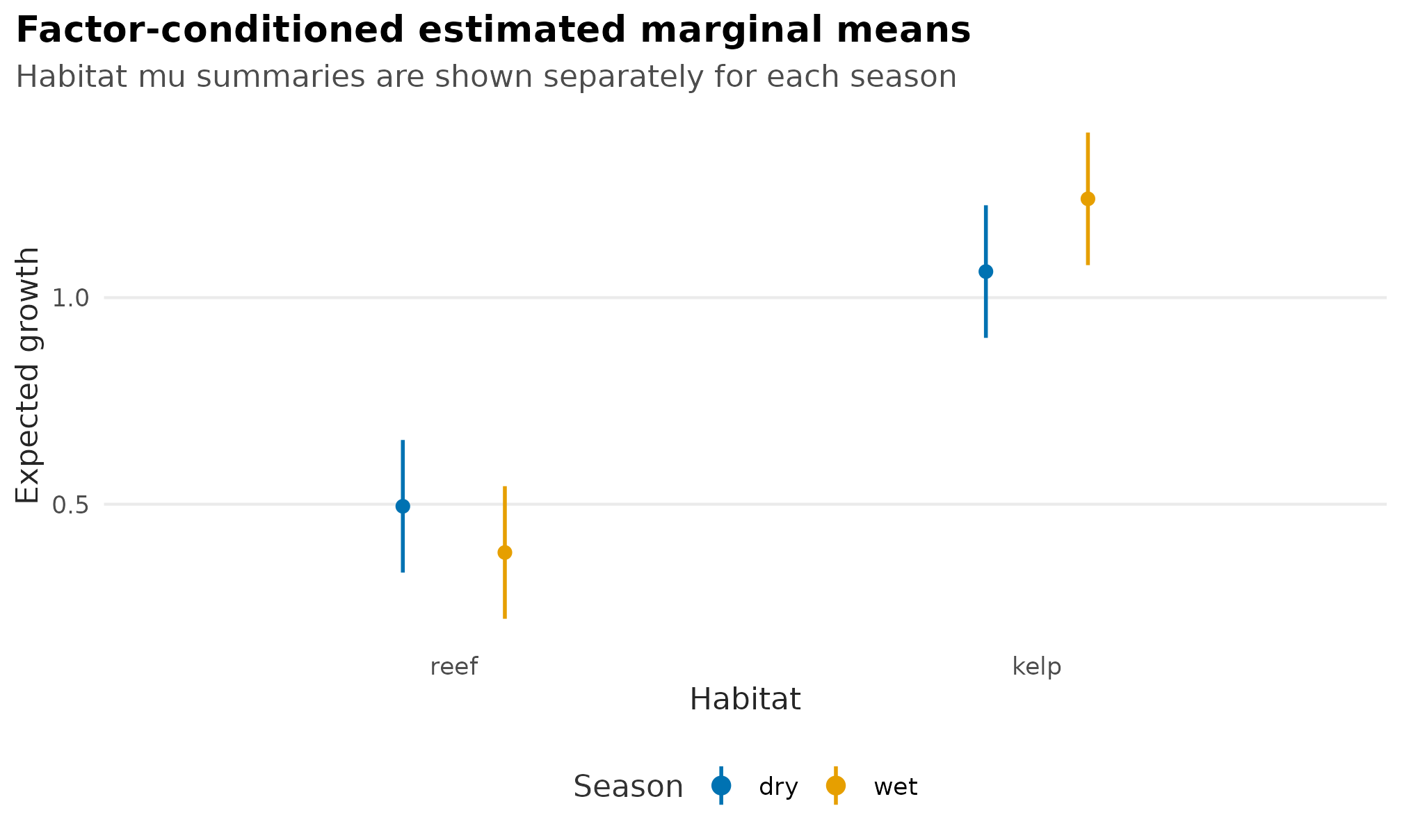
Season-conditioned estimated marginal mean mu summaries;
intervals come from the emmeans fixed-effect reference
grid.
For a numeric interaction, use an explicit reference grid. Here
temperature is held at three named values so the habitat
contrast does not hide the conditioning rule.
emm_temperature <- suppressMessages(
  as.data.frame(
    emmeans::emmeans(
      fit_growth,
      ~ habitat | temperature,
      at = list(temperature = c(-1, 0, 1)),
      type = "response"
    )
  )
)
emm_temperature$temperature_slice <- factor(
  emm_temperature$temperature,
  levels = c(-1, 0, 1),
  labels = c("cooler", "average", "warmer")
)

ggplot(emm_temperature, aes(temperature_slice, emmean, colour = habitat)) +
  geom_line(
    aes(group = habitat),
    linewidth = 0.65,
    alpha = 0.85
  ) +
  geom_errorbar(
    aes(ymin = asymp.LCL, ymax = asymp.UCL),
    width = 0.08,
    linewidth = 0.65
  ) +
  geom_point(size = 2.5) +
  scale_drmtmb_colour +
  labs(
    title = "Marginal means across temperature slices",
    subtitle = "The same fixed-effect mu bridge, evaluated at named temperature slices",
    x = "Temperature slice",
    y = "Expected growth",
    colour = "Habitat"
  ) +
  theme_point_interval_gallery()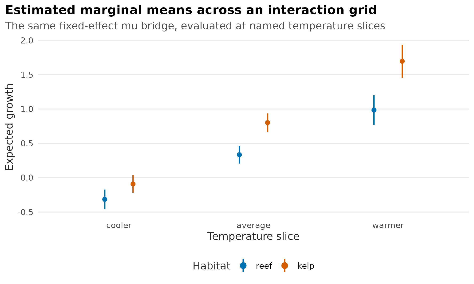
Estimated marginal mean mu trends for habitat across three
named temperature values; intervals are fixed-effect
emmeans intervals.
Empirical marginal summaries use a different rule.
prediction_grid(..., margin = "empirical") crosses a focal
value with fitted rows, and marginal_parameters() averages
the resulting parameter predictions. The helper itself is still a
plug-in point summary, so the interval bars below are a display
approximation: they average row-wise Wald prediction limits from
predict_parameters(conf.int = TRUE) within each
habitat.
empirical_habitat_grid <- prediction_grid(
  fit_growth,
  focal = "habitat",
  at = list(habitat = levels(fish$habitat)),
  margin = "empirical"
)
empirical_habitat <- marginal_parameters(
  fit_growth,
  newdata = empirical_habitat_grid,
  dpar = "mu",
  by = "habitat"
)
empirical_habitat_rowwise <- predict_parameters(
  fit_growth,
  newdata = empirical_habitat_grid,
  dpar = "mu",
  conf.int = TRUE
)
empirical_habitat_wald <- aggregate(
  cbind(conf.low, conf.high) ~ habitat,
  data = empirical_habitat_rowwise,
  FUN = mean
)
empirical_habitat_plot <- empirical_habitat
empirical_habitat_plot$conf.low <- empirical_habitat_wald$conf.low[
  match(empirical_habitat_plot$habitat, empirical_habitat_wald$habitat)
]
empirical_habitat_plot$conf.high <- empirical_habitat_wald$conf.high[
  match(empirical_habitat_plot$habitat, empirical_habitat_wald$habitat)
]
empirical_habitat_plot$conf.status <- "wald"
empirical_habitat_plot$interval_source <- "averaged_rowwise_wald"

ggplot(empirical_habitat_rowwise, aes(habitat, estimate, fill = habitat)) +
  geom_violin(
    width = 0.55,
    alpha = 0.16,
    colour = NA,
    trim = FALSE
  ) +
  geom_point(
    aes(colour = habitat),
    position = position_jitter(width = 0.08, height = 0),
    alpha = 0.22,
    size = 0.65,
    show.legend = FALSE
  ) +
  geom_errorbar(
    data = empirical_habitat_plot,
    aes(
      y = estimate,
      ymin = conf.low,
      ymax = conf.high,
      colour = habitat
    ),
    width = 0.10,
    linewidth = 0.7
  ) +
  geom_point(
    data = empirical_habitat_plot,
    aes(y = estimate, colour = habitat),
    size = 2.4
  ) +
  scale_drmtmb_colour +
  scale_drmtmb_fill +
  labs(
    title = "Empirical marginal mu summary",
    subtitle = "Large points are plug-in means; bars average row-wise Wald limits",
    x = NULL,
    y = "Expected growth",
    colour = "Habitat",
    fill = "Habitat"
  ) +
  guides(colour = "none", fill = "none") +
  theme_drmtmb_gallery()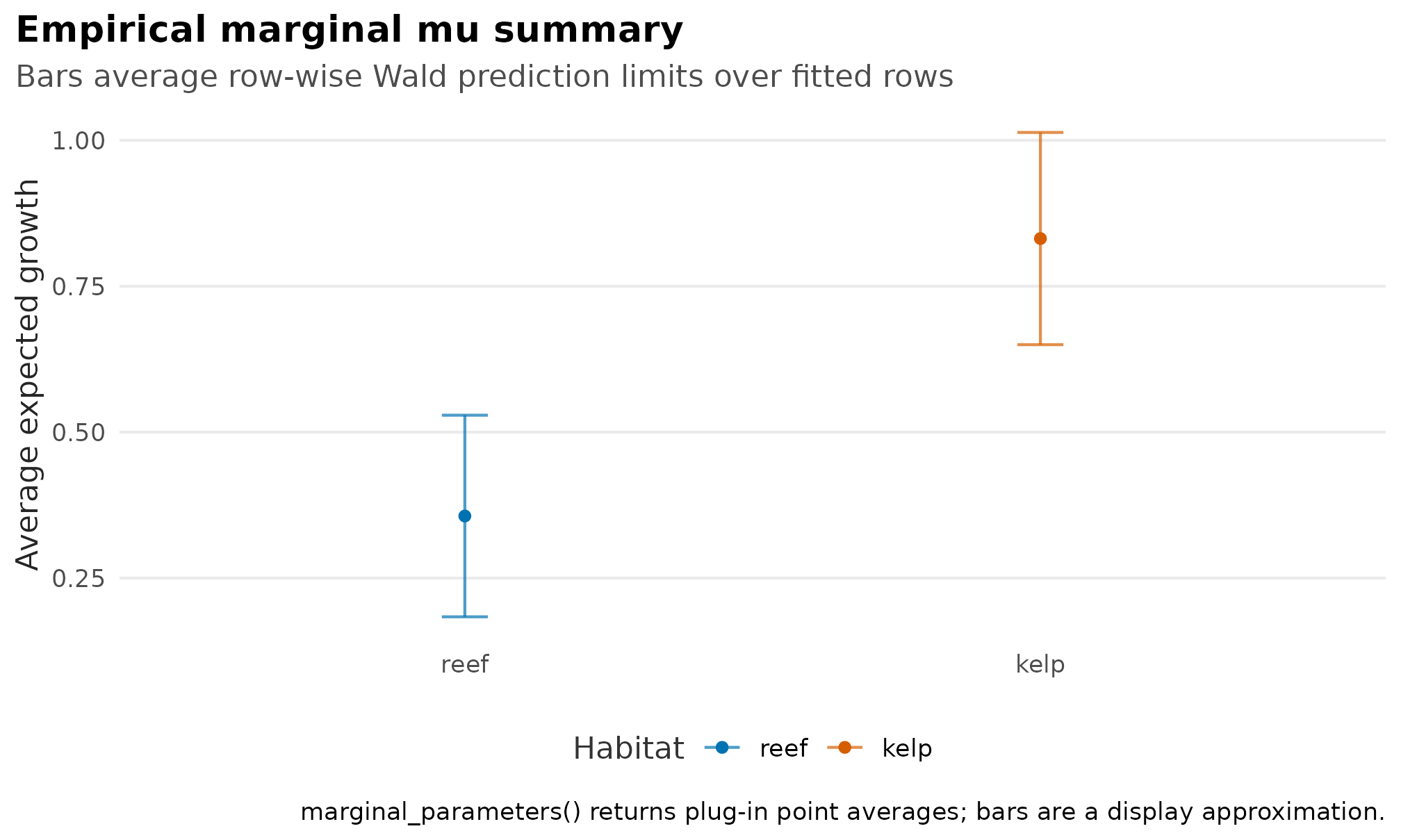
Empirical marginal mu summaries by habitat; faint marks are
fitted-row predictions, large points are plug-in marginal means, and
bars average row-wise Wald limits as a display approximation.
Unsupported targets should be visible before a reader tries to plot
them. The current emmeans bridge is for fixed-effect
univariate mu; other targets should use parameter
prediction, corpairs(), profile intervals, or a future
feature-specific design.
emmeans_boundary <- data.frame(
  target = c(
    "Fixed-effect univariate mu",
    "sigma",
    "Bivariate responses",
    "Zero-inflated or hurdle means",
    "Ordinal expected scores",
    "Random-effect targets"
  ),
  status = c(
    "Supported emmeans route",
    "Unsupported boundary",
    "Unsupported boundary",
    "Unsupported boundary",
    "Unsupported boundary",
    "Unsupported boundary"
  )
)
emmeans_boundary$route <- c(
  "supported EMMs",
  "predict_parameters()",
  "separate bivariate design",
  "family-specific marginal route",
  "ordinal support later",
  "ranef(), profile_targets()"
)
emmeans_boundary$target <- factor(
  emmeans_boundary$target,
  levels = rev(emmeans_boundary$target)
)
emmeans_boundary$status <- factor(
  emmeans_boundary$status,
  levels = c("Supported emmeans route", "Unsupported boundary")
)
emmeans_boundary$status_label <- ifelse(
  emmeans_boundary$status == "Supported emmeans route",
  "supported",
  "boundary"
)

ggplot(emmeans_boundary, aes(y = target)) +
  geom_segment(
    aes(x = 0.92, xend = 2.35, yend = target),
    colour = "grey86",
    linewidth = 0.35
  ) +
  geom_point(
    aes(x = 1, fill = status),
    shape = 21,
    size = 3.4,
    colour = "white",
    stroke = 0.8
  ) +
  geom_text(
    aes(x = 1.14, label = status_label, colour = status),
    hjust = 0,
    size = 2.85,
    fontface = "bold"
  ) +
  geom_text(
    aes(x = 1.65, label = route),
    hjust = 0,
    size = 2.75,
    colour = "grey25"
  ) +
  scale_fill_manual(values = c(
    "Supported emmeans route" = "#0072B2",
    "Unsupported boundary" = "#E69F00"
  )) +
  scale_colour_manual(values = c(
    "Supported emmeans route" = "#0072B2",
    "Unsupported boundary" = "#8A5700"
  )) +
  scale_x_continuous(
    limits = c(0.86, 2.55),
    breaks = c(1.14, 1.65),
    labels = c("Status", "Current route")
  ) +
  labs(
    title = "Current emmeans support boundary",
    subtitle = "Only fixed-effect univariate mu is advertised as an emmeans target",
    x = NULL,
    y = NULL,
    fill = "Status"
  ) +
  theme_drmtmb_gallery() +
  theme(
    axis.text.x = element_text(size = 8.8, face = "bold", colour = "grey35"),
    axis.ticks.x = element_blank(),
    panel.grid = element_blank(),
    legend.position = "none"
  )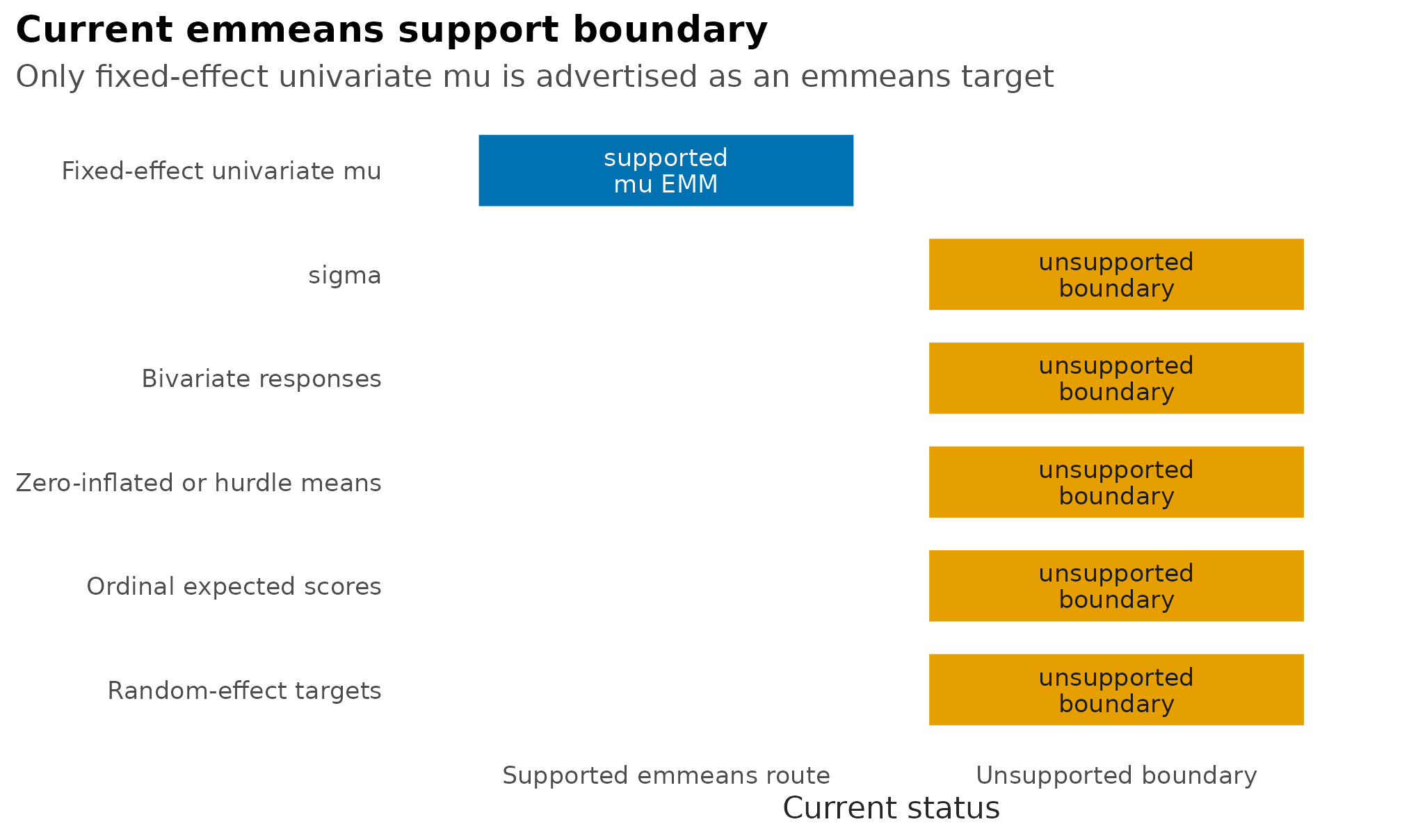
Support-boundary strip for emmeans; fixed-effect univariate
mu is supported, while other targets show the fitted route
to use instead.
Continuous by continuous interaction
For two continuous predictors, choose scientifically meaningful slices of one predictor and show fitted slopes across the other. The values should be named in the legend so the reader can interpret the conditioning.
set.seed(2593)
n_cc <- 180
soil <- data.frame(
  temperature = runif(n_cc, -1.5, 1.5),
  moisture = runif(n_cc, -1.4, 1.4)
)
soil$growth <- rnorm(
  n_cc,
  mean = 0.3 +
    0.55 * soil$temperature +
    0.45 * soil$moisture -
    0.35 * soil$temperature * soil$moisture,
  sd = 0.45
)

fit_cont_cont <- drmTMB(
  bf(growth ~ temperature * moisture, sigma ~ 1),
  family = gaussian(),
  data = soil
)

grid_cont_cont <- expand.grid(
  temperature = seq(-1.5, 1.5, length.out = 80),
  moisture = c(-1, 0, 1)
)
grid_cont_cont$moisture_level <- factor(
  grid_cont_cont$moisture,
  levels = c(-1, 0, 1),
  labels = c("low moisture", "average moisture", "high moisture")
)

pred_cont_cont <- predict_parameters(
  fit_cont_cont,
  newdata = grid_cont_cont,
  dpar = "mu",
  conf.int = TRUE
)

ggplot(
  pred_cont_cont,
  aes(temperature, estimate, colour = moisture_level, fill = moisture_level)
) +
  geom_point(
    data = soil,
    aes(temperature, growth),
    inherit.aes = FALSE,
    alpha = 0.18,
    size = 1,
    colour = "grey35"
  ) +
  geom_ribbon(aes(ymin = conf.low, ymax = conf.high), alpha = 0.14, colour = NA) +
  geom_line(linewidth = 0.8) +
  scale_colour_manual(values = c(
    "low moisture" = gallery_colour("blue"),
    "average moisture" = gallery_colour("green"),
    "high moisture" = gallery_colour("orange")
  )) +
  scale_fill_manual(values = c(
    "low moisture" = gallery_colour("blue"),
    "average moisture" = gallery_colour("green"),
    "high moisture" = gallery_colour("orange")
  )) +
  labs(
    title = "Continuous by continuous interaction",
    subtitle = "Ribbons are 95% Wald bands at three moisture slices",
    x = "Temperature anomaly",
    y = "Growth",
    colour = "Moisture slice",
    fill = "Moisture slice"
  ) +
  theme_drmtmb_gallery()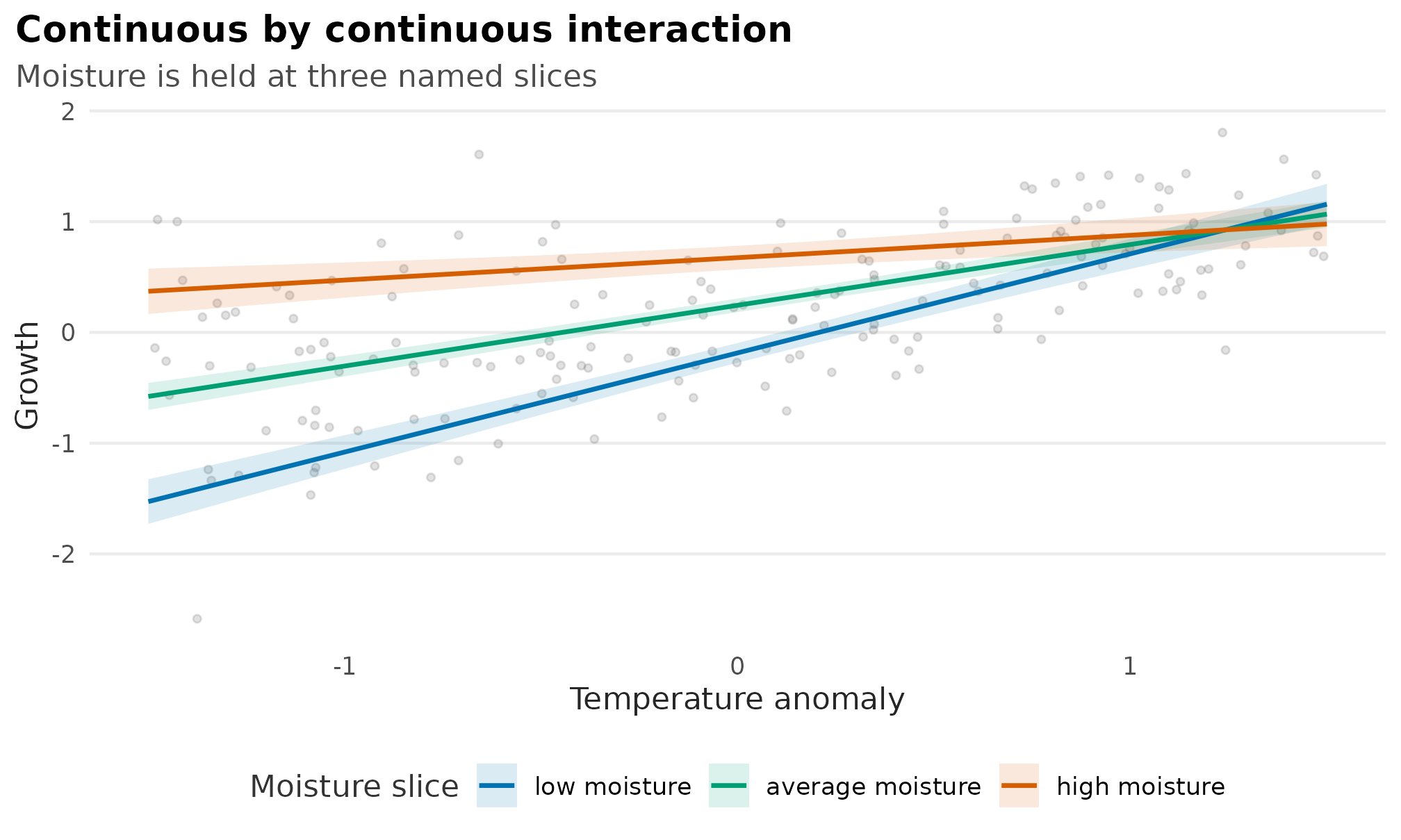
Continuous-by-continuous fitted mu interaction over raw
observations; ribbons are 95% Wald confidence bands at low, average, and
high moisture.
The raw point cloud is not coloured by the sliced predictor because the fitted lines are conditional displays, not clusters in the data. This keeps the visual message honest: the model is being read at three moisture values, while the observations span the whole moisture gradient.
Correlation summaries
Correlation displays should keep layers separate. Residual
rho12, ordinary-group correlations, phylogenetic
correlations, coordinate-spatial correlations, animal-model
correlations, and lower-level relmat() correlations are not
the same parameter even when all are correlations. A fitted workflow
should start from corpairs(fit) and keep the interval
provenance columns.
This section has two figures and they are not the same kind of object. The first is fitted: it comes from a model in this document, and its interval was computed. The second is an illustrative layout fixture with typed numbers, included to show a multi-layer arrangement the package cannot yet produce from a single fit. The distinction is stated in each caption; do not read the second as a result.
Fitted correlation summary
corpairs() returns one row per correlation with the
provenance columns attached, and plot_corpairs() draws the
Confidence Eye from that table. The interval below is a
profile-likelihood interval, so conf.status and
interval_source both read profile.
The fit uses a constant residual correlation, rho12 ~ 1.
That is deliberate: when rho12 is modelled as a regression,
corpairs(conf.int = TRUE) reports
conf.status = "newdata_required" and returns no bounds,
because there is no single scalar correlation to profile. That status is
an instruction, not a dead end. Supply the covariate values you want and
the interval is computed per row, either as a profile interval from
confint(fit, parm = "rho12", newdata = grid, method = "profile")
or as a Wald interval from
predict_parameters(fit, newdata = grid, dpar = "rho12", conf.int = TRUE).
The constant rho12 ~ 1 profile interval is a finite
computed reporting interval, but its coverage has not been certified;
the row-specific intervals are likewise computed without established
coverage.
fit_pair_const <- drmTMB(
  bf(
    mu1 = activity ~ disturbance,
    mu2 = boldness ~ disturbance,
    sigma1 ~ 1,
    sigma2 ~ 1,
    rho12 ~ 1
  ),
  family = c(gaussian(), gaussian()),
  data = pair_dat
)

pair_fitted <- corpairs(fit_pair_const, conf.int = TRUE)
pair_fitted[, c(
  "level", "parameter", "estimate",
  "conf.low", "conf.high", "conf.status", "interval_source"
)]
#>      level parameter   estimate   conf.low   conf.high conf.status
#> 1 residual     rho12 -0.1899323 -0.3341724 -0.03699916     profile
#>   interval_source
#> 1         profile

plot_corpairs(pair_fitted) +
  theme_drmtmb_gallery() +
  theme(legend.position = "none")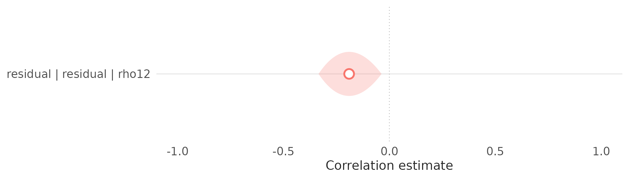
Fitted residual correlation from corpairs() with its
profile-likelihood interval, drawn by plot_corpairs(); this
row is computed from a model in this document.
One fitted row, one computed interval. Compare the
interval_source column here with the figure that
follows.
Illustrative multi-layer layout (fixture, not fitted)
A Confidence Eye should appear only when finite interval bounds
exist. The compact example below is a hand-specified
fixture: the estimates and bounds are typed constants, not
model output. It exists to show how several correlation layers would be
arranged in one display, which no single drmTMB fit
currently produces. The pale eye is a 95% region shaped on Fisher’s
z scale; the hollow circle marks the estimate. Rows without
finite bounds should remain point-only diagnostics, and the plot should
not invent an eye.
Its interval_source column reads
illustrative_profile rather than profile,
which is the tell that separates it from the fitted figure above. Treat
every number in it as a layout placeholder.
pair_table <- data.frame(
  level = c("residual", "group", "phylogenetic", "spatial", "animal", "relmat"),
  class = c(
    "residual",
    "intercept-slope",
    "location-location",
    "location-location",
    "location-location",
    "location-location"
  ),
  parameter = c(
    "rho12",
    "cor((Intercept), x | id)",
    "cor(mu1, mu2 | phylo)",
    "cor(mu1, mu2 | spatial)",
    "cor(mu1, mu2 | animal)",
    "cor(mu1, mu2 | relmat)"
  ),
  estimate = c(-0.32, 0.44, 0.61, 0.38, 0.52, -0.27),
  modelled = rep(TRUE, 6),
  conf.low = c(-0.54, 0.12, 0.32, 0.05, 0.18, -0.58),
  conf.high = c(-0.05, 0.68, 0.80, 0.63, 0.75, 0.10),
  conf.status = rep("illustrative", 6),
  interval_source = rep("illustrative_profile", 6),
  display = c(
    "Residual\nrho12",
    "Group\nintercept-slope",
    "Phylogenetic\nlocation-location",
    "Spatial\nlocation-location",
    "Animal\nlocation-location",
    "relmat\nlocation-location"
  ),
  stringsAsFactors = FALSE
)
pair_table$row_id <- rev(seq_len(nrow(pair_table)))
pair_table$has_interval <- is.finite(pair_table$conf.low) &
  is.finite(pair_table$conf.high)
correlation_palette <- c(
  "residual" = gallery_colour("blue"),
  "group" = gallery_colour("green"),
  "phylogenetic" = gallery_colour("orange"),
  "spatial" = gallery_colour("sky"),
  "animal" = gallery_colour("pink"),
  "relmat" = gallery_colour("charcoal")
)
make_correlation_confidence_eye <- function(row, level = 0.95, n = 240) {
  if (!all(is.finite(c(row$estimate, row$conf.low, row$conf.high)))) {
    return(data.frame())
  }
  z_estimate <- atanh(guard_rho(row$estimate))
  z_low <- atanh(guard_rho(row$conf.low))
  z_high <- atanh(guard_rho(row$conf.high))
  z_cutoff <- qnorm(1 - (1 - level) / 2)
  z_se <- max((z_high - z_low) / (2 * z_cutoff), .Machine$double.eps)
  cutoff <- 0.5 * qchisq(level, df = 1)
  z <- seq(
    z_estimate - sqrt(2 * cutoff) * z_se,
    z_estimate + sqrt(2 * cutoff) * z_se,
    length.out = n
  )
  rho <- tanh(z)
  height <- pmax(cutoff - 0.5 * ((z - z_estimate) / z_se)^2, 0) /
    cutoff * 0.17
  data.frame(
    rho = rho,
    height = height,
    ymin = row$row_id - height,
    ymax = row$row_id + height,
    row_id = row$row_id,
    display = row$display,
    level = row$level
  )
}
correlation_cloud <- do.call(
  rbind,
  lapply(seq_len(nrow(pair_table)), function(i) make_correlation_confidence_eye(pair_table[i, ]))
)

ggplot() +
  geom_vline(
    xintercept = seq(-1, 1, by = 0.5),
    colour = "grey90",
    linewidth = 0.35
  ) +
  geom_vline(xintercept = 0, colour = "grey55", linewidth = 0.55, linetype = "dotted") +
  geom_ribbon(
    data = correlation_cloud,
    aes(
      rho,
      ymin = ymin,
      ymax = ymax,
      fill = level,
      group = interaction(level, display)
    ),
    alpha = 0.24,
    colour = NA
  ) +
  geom_point(
    data = pair_table,
    aes(estimate, row_id, colour = level),
    shape = 21,
    fill = "white",
    size = 3.1,
    stroke = 1.1,
    inherit.aes = FALSE
  ) +
  scale_colour_manual(values = correlation_palette) +
  scale_fill_manual(values = correlation_palette, guide = "none") +
  scale_x_continuous(
    limits = c(-1, 1),
    breaks = seq(-1, 1, by = 0.5),
    expand = expansion(mult = 0.04)
  ) +
  scale_y_continuous(
    breaks = pair_table$row_id,
    labels = pair_table$display,
    expand = expansion(add = 0.42)
  ) +
  labs(
    title = "ILLUSTRATIVE FIXTURE - not a fitted result",
    subtitle = paste(
      "Estimates and bounds are typed constants showing layout only.",
      "No drmTMB fit produces these six rows together."
    ),
    x = "Correlation estimate",
    y = NULL,
    colour = NULL
  ) +
  theme_drmtmb_gallery() +
  theme(
    axis.text.y = element_text(size = 10.5, colour = "grey30"),
    axis.ticks.y = element_blank(),
    axis.line.x = element_line(colour = "grey35", linewidth = 0.35),
    axis.ticks.x = element_line(colour = "grey35", linewidth = 0.35),
    axis.ticks.length.x = grid::unit(3, "pt"),
    panel.grid = element_blank()
  ) +
  guides(colour = "none", fill = "none")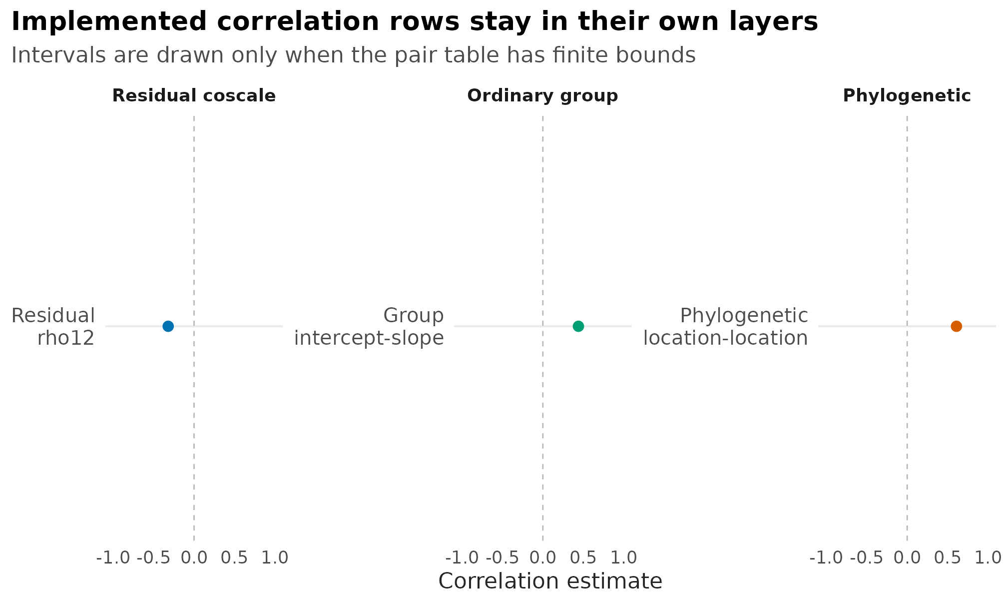
FIXTURE, NOT FITTED: illustrative multi-layer correlation layout with hand-typed estimates and bounds; shown to demonstrate arrangement only, and no value here is a model result.
The figure should be read as an uncertainty display, not as a new model class. Rows with finite bounds get default Confidence Eyes. Rows without finite bounds should be shown as point-only diagnostics. This prevents the plot from implying uncertainty evidence that the fitted object or extractor did not provide.
layer_boundary <- expand.grid(
  layer = c(
    "Residual rho12",
    "Ordinary group",
    "Phylogenetic",
    "Spatial",
    "Animal",
    "relmat"
  ),
  target = c("Constant q2 row", "Regression or q4/scale extension"),
  stringsAsFactors = FALSE
)
layer_boundary$support <- "Planned"
layer_boundary$support[
  layer_boundary$target == "Constant q2 row" &
    layer_boundary$layer %in% c(
      "Residual rho12",
      "Ordinary group",
      "Phylogenetic",
      "Spatial",
      "Animal",
      "relmat"
    )
] <- "Fitted q2"
layer_boundary$support[
  layer_boundary$target == "Regression or q4/scale extension" &
    layer_boundary$layer %in% c("Spatial", "Animal", "relmat")
] <- "Partial q4"
layer_boundary$support <- factor(
  layer_boundary$support,
  levels = c("Fitted q2", "Partial q4", "Planned")
)
layer_boundary$layer <- factor(
  layer_boundary$layer,
  levels = c(
    "Residual rho12",
    "Ordinary group",
    "Phylogenetic",
    "Spatial",
    "Animal",
    "relmat"
  )
)
layer_boundary$target <- factor(
  layer_boundary$target,
  levels = c("Constant q2 row", "Regression or q4/scale extension")
)
ggplot(layer_boundary, aes(target, layer, fill = support)) +
  geom_tile(colour = "white", linewidth = 1) +
  geom_text(aes(label = support), size = 2.8, colour = "white", fontface = "bold") +
  scale_fill_manual(
    values = c(
      "Fitted q2" = gallery_colour("green"),
      "Partial q4" = gallery_colour("orange"),
      "Planned" = gallery_colour("charcoal")
    )
  ) +
  labs(
    title = "Correlation layers have different support boundaries",
    subtitle = "q2 constants are separate from richer regression and q4 extensions",
    x = NULL,
    y = NULL,
    fill = "Status"
  ) +
  theme_drmtmb_gallery() +
  theme(
    panel.grid = element_blank(),
    legend.position = "none"
  )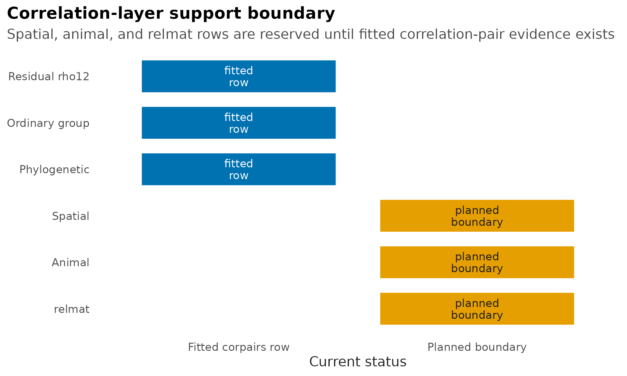
Support-boundary strip for correlation layers; fitted q=2 rows, partial
richer q=4 or regression rows, and planned residual-rho12
routes are kept separate.
The grid prevents a common mistake: seeing one fitted correlation route and assuming all correlation layers now share the same regression and q4 support.
Simulation operating characteristics
Simulation figures answer different questions from model-interpretation figures. They should show bias, error, coverage, runtime, and failures beside the model surface being tested.
sim_targets <- data.frame(
  surface = rep(
    c("Gaussian location-scale", "Proportion", "Count"),
    each = 4
  ),
  estimand = rep(c("beta_x", "sigma", "sd_intercept", "rho12"), 3),
  bias = c(
    0.01, -0.02, 0.04, 0.00,
    -0.01, 0.03, NA, NA,
    0.02, -0.01, -0.04, NA
  ),
  rmse = c(
    0.07, 0.09, 0.13, 0.11,
    0.08, 0.10, NA, NA,
    0.10, 0.09, 0.16, NA
  ),
  coverage = c(
    0.95, 0.94, 0.91, 0.93,
    0.94, 0.92, NA, NA,
    0.93, 0.95, 0.89, NA
  )
)
sim_targets$n_rep <- 500L
sim_targets$error_sd <- sqrt(
  pmax(sim_targets$rmse^2 - sim_targets$bias^2, 0)
)
sim_bias_rows <- do.call(
  rbind,
  lapply(seq_len(nrow(sim_targets)), function(i) {
    row <- sim_targets[i, ]
    if (is.na(row$bias) || is.na(row$rmse)) {
      return(NULL)
    }
    data.frame(
      surface = row$surface,
      estimand = row$estimand,
      replicate = seq_len(row$n_rep),
      bias_error = row$bias +
        qnorm(ppoints(row$n_rep)) * row$error_sd
    )
  })
)
summarise_bias_rows <- function(rows) {
  data.frame(
    surface = rows$surface[1],
    estimand = rows$estimand[1],
    bias = mean(rows$bias_error),
    rmse = sqrt(mean(rows$bias_error^2)),
    error_sd = stats::sd(rows$bias_error),
    n_rep = nrow(rows)
  )
}
sim_summary <- do.call(
  rbind,
  lapply(
    split(
      sim_bias_rows,
      interaction(sim_bias_rows$surface, sim_bias_rows$estimand, drop = TRUE)
    ),
    summarise_bias_rows
  )
)
sim_summary <- merge(
  sim_targets[c("surface", "estimand", "coverage")],
  sim_summary,
  by = c("surface", "estimand"),
  all.x = TRUE,
  sort = FALSE
)
sim_summary$n_rep <- 500L
sim_summary$bias_mcse <- sim_summary$error_sd / sqrt(sim_summary$n_rep)
sim_summary$bias_low <- sim_summary$bias - 1.96 * sim_summary$bias_mcse
sim_summary$bias_high <- sim_summary$bias + 1.96 * sim_summary$bias_mcse
sim_summary$coverage_mcse <- sqrt(
  sim_summary$coverage * (1 - sim_summary$coverage) / sim_summary$n_rep
)
sim_summary$coverage_low <- pmax(
  0,
  sim_summary$coverage - 1.96 * sim_summary$coverage_mcse
)
sim_summary$coverage_high <- pmin(
  1,
  sim_summary$coverage + 1.96 * sim_summary$coverage_mcse
)
sim_summary$surface <- factor(
  sim_summary$surface,
  levels = names(surface_palette)
)
estimand_labels <- c(
  "beta_x" = "beta_x fixed slope",
  "sigma" = "sigma residual SD",
  "sd_intercept" = "sd_intercept group SD",
  "rho12" = "rho12 residual correlation"
)
sim_summary$estimand_label <- factor(
  estimand_labels[sim_summary$estimand],
  levels = rev(unname(estimand_labels))
)
surface_facet_labels <- c(
  "Gaussian location-scale" = "Gaussian\nlocation-scale",
  "Proportion" = "Proportion",
  "Count" = "Count"
)
display_replicates <- 55
sim_rain <- do.call(
  rbind,
  lapply(split(sim_bias_rows, sim_bias_rows[c("surface", "estimand")]), function(rows) {
    if (nrow(rows) == 0L) {
      return(NULL)
    }
    keep <- round(seq(1, nrow(rows), length.out = display_replicates))
    rows[keep, , drop = FALSE]
  })
)
sim_rain$surface <- factor(sim_rain$surface, levels = levels(sim_summary$surface))
sim_rain$estimand_label <- factor(
  estimand_labels[sim_rain$estimand],
  levels = levels(sim_summary$estimand_label)
)
sim_bias_missing <- sim_summary[is.na(sim_summary$bias), , drop = FALSE]

ggplot(sim_rain, aes(bias_error, estimand_label)) +
  geom_vline(xintercept = 0, linetype = "dotted", colour = "grey60") +
  geom_violin(
    aes(
      fill = surface
    ),
    width = 0.62,
    alpha = 0.16,
    colour = NA,
    scale = "width",
    trim = FALSE
  ) +
  geom_point(
    aes(colour = surface),
    position = position_jitter(height = 0.05, width = 0),
    alpha = 0.22,
    size = 0.75,
    show.legend = FALSE
  ) +
  geom_errorbar(
    data = sim_summary,
    aes(
      xmin = bias_low,
      xmax = bias_high,
      y = estimand_label,
      colour = surface
    ),
    inherit.aes = FALSE,
    orientation = "y",
    width = 0.16,
    linewidth = 0.65,
    na.rm = TRUE
  ) +
  geom_point(
    data = sim_summary,
    aes(bias, estimand_label, colour = surface),
    size = 2.6,
    na.rm = TRUE
  ) +
  geom_text(
    data = sim_bias_missing,
    aes(x = -0.47, y = estimand_label, label = "not\ntargeted"),
    colour = "grey55",
    size = 2.25,
    lineheight = 0.9,
    hjust = 0,
    inherit.aes = FALSE
  ) +
  facet_wrap(
    ~surface,
    nrow = 1,
    labeller = labeller(surface = as_labeller(surface_facet_labels))
  ) +
  scale_colour_manual(values = surface_palette, drop = FALSE) +
  scale_fill_manual(values = surface_palette, drop = FALSE) +
  labs(
    title = "ILLUSTRATIVE FIXTURE - not a simulation result",
    subtitle = paste(
      "Bias by estimand. Every value is a typed constant, not a fitted or",
      "simulated estimate.\nLarge points and bars show mean bias with 95% MCSE",
      "intervals over the fixture replicates."
    ),
    x = "Estimate minus truth",
    y = NULL,
    colour = "Surface"
  ) +
  guides(fill = "none", colour = "none") +
  theme_drmtmb_gallery()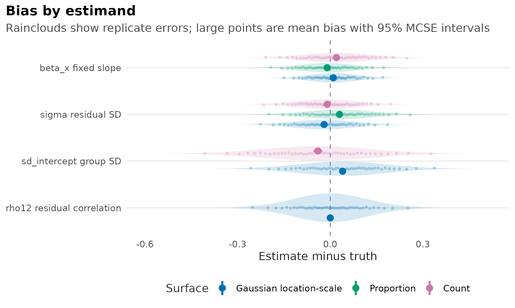
Simulation grammar fixture showing replicate-error bias clouds with MCSE intervals and coverage block proportions with binomial MCSE whiskers.
sim_coverage_present <- sim_summary[!is.na(sim_summary$coverage), , drop = FALSE]
sim_coverage_present$y_id <- as.numeric(sim_coverage_present$estimand_label)
make_coverage_blocks <- function(row, n_block = 18) {
  block_size <- max(8L, floor(row$n_rep / n_block))
  block_coverage <- qbinom(
    ppoints(n_block),
    size = block_size,
    prob = row$coverage
  ) / block_size
  data.frame(
    surface = row$surface,
    estimand_label = row$estimand_label,
    block_coverage = block_coverage
  )
}
sim_coverage_blocks <- do.call(
  rbind,
  lapply(seq_len(nrow(sim_coverage_present)), function(i) {
    make_coverage_blocks(sim_coverage_present[i, ])
  })
)
sim_coverage_missing <- sim_summary[is.na(sim_summary$coverage), , drop = FALSE]

ggplot(sim_coverage_present, aes(coverage, estimand_label, colour = surface)) +
  geom_vline(xintercept = 0.95, linetype = "dotted", colour = "grey60") +
  geom_point(
    data = sim_coverage_blocks,
    aes(block_coverage, estimand_label, colour = surface),
    position = position_jitter(height = 0.07, width = 0),
    alpha = 0.20,
    size = 0.75,
    inherit.aes = FALSE
  ) +
  geom_errorbar(
    aes(xmin = coverage_low, xmax = coverage_high, colour = surface),
    orientation = "y",
    width = 0.18,
    linewidth = 0.45,
    na.rm = TRUE
  ) +
  geom_point(size = 2.3, na.rm = TRUE) +
  geom_text(
    data = sim_coverage_missing,
    aes(x = 0.755, y = estimand_label, label = "not\ntargeted"),
    colour = "grey55",
    size = 2.25,
    lineheight = 0.9,
    hjust = 0,
    inherit.aes = FALSE
  ) +
  facet_wrap(
    ~surface,
    nrow = 1,
    labeller = labeller(surface = as_labeller(surface_facet_labels))
  ) +
  coord_cartesian(xlim = c(0.75, 1)) +
  scale_x_continuous(
    breaks = c(0.75, 0.85, 0.95),
    labels = c("0.75", "0.85", "0.95")
  ) +
  scale_colour_manual(values = surface_palette, drop = FALSE) +
  labs(
    title = "ILLUSTRATIVE FIXTURE - not a simulation result",
    subtitle = paste(
      "Interval coverage. Every value is a typed constant, not a fitted or",
      "simulated estimate.\nLarge points and bars show 95% binomial MCSE over",
      "the fixture replicate blocks."
    ),
    x = "Empirical coverage",
    y = NULL,
    colour = "Surface"
  ) +
  guides(colour = "none") +
  theme_drmtmb_gallery()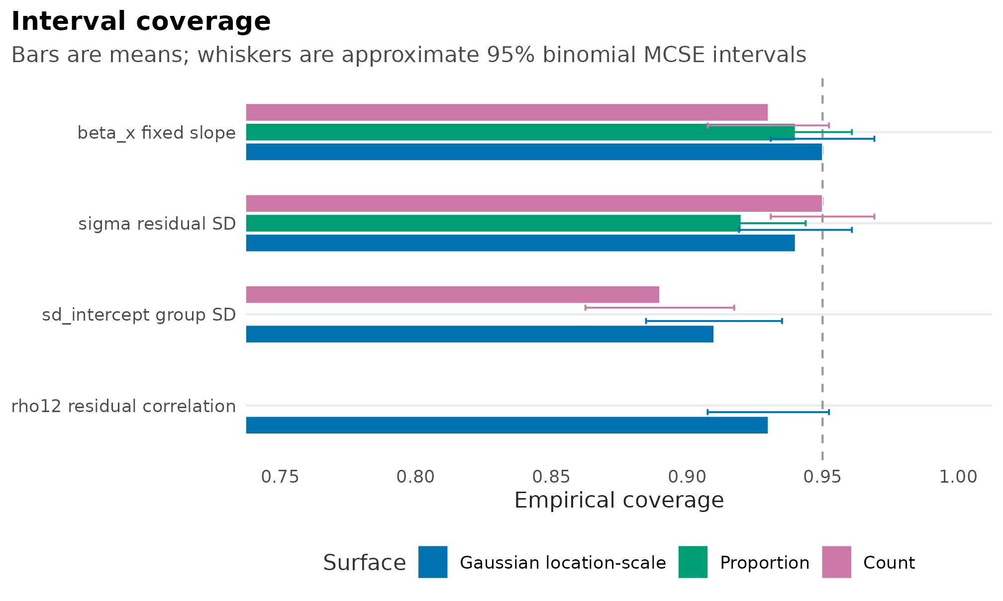
Simulation grammar fixture showing replicate-error bias clouds with MCSE intervals and coverage block proportions with binomial MCSE whiskers.
These figures use a small illustrative table with the same columns
that simulation summaries should carry. The bias panel shows the
intended raincloud-style grammar: real reports should draw the
replicate-level errors, then overplot the mean and MCSE interval for
each defined surface-estimand cell. The panel still leaves estimands
disconnected because beta_x, sigma,
sd_intercept, and rho12 are categorical
targets, not steps along one trajectory. The coverage panel uses the
more utilitarian simulation grammar: replicate or replicate-block
proportions first, then aggregate coverage and a 95% binomial MCSE
interval. This small fixture illustrates block points; formal simulation
reports should use the stored replicate rows or stored block summaries
rather than reconstructing raw uncertainty from aggregate CSVs alone.
The comprehensive simulation programme should not be count-only. It
should add continuous, meta-analysis, proportion, count, ordinal,
bivariate, random-slope, and structured-dependence surfaces as each
surface becomes ready. Real simulation reports should also show the run
manifest and warning/error ledger so missing or failed fits are not
hidden behind clean-looking panels.
Gallery source map
The gallery is easier to audit when every figure names its source object, extractor, interval source, and support boundary. Use this table as a quick check before adapting a plot to a manuscript, tutorial, or simulation report.
gallery_source_map <- data.frame(
  figure = c(
    "Mean with confidence band",
    "mu and sigma surfaces",
    "Observed vs implied residual scale",
    "Fixed-effect slope Confidence Eye",
    "nu, zi, and rho12 panels",
    "Worm plot, adequate model",
    "Worm plot, mis-specified sigma",
    "QQ plot, adequate model",
    "Conditional centile chart",
    "Profile-likelihood curve",
    "Variance-component Confidence Eye",
    "Mixed-parameter Confidence Eye",
    "Conditional random-slope modes",
    "sd(site) surface",
    "Discrete habitat comparison",
    "Categorical interaction",
    "Simple emmeans display",
    "Factor-conditioned emmeans grid",
    "Interaction emmeans grid",
    "Empirical marginal mu summary",
    "emmeans support boundary",
    "Continuous interaction",
    "Fitted correlation row",
    "Correlation layout FIXTURE (not fitted)",
    "Correlation support boundary",
    "Simulation bias and coverage FIXTURE"
  ),
  source = c(
    "fit_growth",
    "fit_growth",
    "fit_growth",
    "fit_growth",
    "fit_tail, fit_zi, fit_pair",
    "fit_growth",
    "fit_mis",
    "fit_growth",
    "fit_growth",
    "fit_growth",
    "fit_re_slopes",
    "fit_re_slopes",
    "fit_re_slopes",
    "fit_site_sd",
    "fit_growth",
    "fit_cat_cat",
    "fit_growth",
    "fit_cat_cat",
    "fit_growth",
    "fit_growth",
    "emmeans_boundary",
    "fit_cont_cont",
    "fit_pair_const",
    "pair_table (typed constants)",
    "layer_boundary",
    "sim_summary (typed constants)"
  ),
  extractor_or_plotter = c(
    "predict_parameters(dpar = \"mu\") + ggplot2",
    "predict_parameters() + plot_parameter_surface()",
    "residuals() + predict_parameters(dpar = c(\"mu\", \"sigma\")) + ggplot2",
    "summary(fit)$coefficients + ggplot2",
    "predict_parameters() + plot_parameter_surface()",
    "worm_plot()",
    "worm_plot()",
    "qq_plot()",
    "centile_chart()",
    "profile() + plot()",
    "summary(fit)$parameters + ggplot2",
    "summary(fit)$coefficients + summary(fit)$parameters + ggplot2",
    "ranef() + ggplot2",
    "prediction_grid() + predict_parameters() + plot_parameter_surface()",
    "predict_parameters(dpar = \"mu\") + plot_parameter_surface()",
    "predict_parameters(dpar = \"mu\") + ggplot2",
    "emmeans::emmeans(type = \"response\") + ggplot2",
    "emmeans::emmeans(~ habitat | season) + ggplot2",
    "emmeans::emmeans(~ habitat | temperature) + ggplot2",
    "prediction_grid(margin = \"empirical\") + marginal_parameters() + predict_parameters()",
    "ggplot2 status strip",
    "predict_parameters(dpar = \"mu\") + ggplot2",
    "corpairs(conf.int = TRUE) + plot_corpairs()",
    "typed corpairs-shaped fixture + ggplot2",
    "ggplot2 status strip",
    "ggplot2 fixture display"
  ),
  interval_source = c(
    "Wald intervals from predict_parameters()",
    "Wald bands from predict_parameters()",
    "No intervals; observed magnitudes against a fitted curve",
    "Wald regions on the fitted parameter scale",
    "Wald intervals from each fitted parameter table",
    "No intervals; qualitative trend only",
    "No intervals; qualitative trend only",
    "No intervals; identity reference line",
    "No intervals; fitted conditional quantiles only",
    "Profile-likelihood interval read from the curve",
    "Wald regions shaped on log-SD scale",
    "Wald regions shaped per parameter class (identity, log-SD, Fisher-z)",
    "No intervals; conditional modes only",
    "conf.status = \"wald_unavailable\"; no band",
    "Wald intervals from predict_parameters()",
    "Wald intervals from predict_parameters()",
    "asymptotic emmeans intervals",
    "asymptotic emmeans intervals",
    "asymptotic emmeans intervals",
    "Plug-in mean; bars average row-wise Wald limits",
    "No intervals; status only",
    "Wald intervals from predict_parameters()",
    "conf.status = \"profile\"; computed profile interval",
    "Typed constants; interval_source = \"illustrative_profile\"",
    "No intervals; status only",
    "Typed constants, not simulation evidence"
  ),
  support_boundary = c(
    "fixed-effect univariate mu",
    "fixed-effect mu and sigma",
    "fixed-effect sigma surface; a display check, not a formal test",
    "fixed-effect mu and sigma slopes",
    "fixed-effect shape, inflation, and residual rho12",
    "randomised quantile residuals; any fitted family",
    "randomised quantile residuals; any fitted family",
    "randomised quantile residuals; any fitted family",
    "fitted conditional quantiles; no centile uncertainty",
    "direct profile targets only; see profile_targets()",
    "ordinary Gaussian random-slope fit",
    "ordinary Gaussian random-slope fit",
    "shrunken deviations, not variance intervals",
    "modelled random-effect SD surface without Wald bands",
    "fixed-effect univariate mu",
    "fixed-effect univariate mu",
    "fixed-effect univariate mu only",
    "fixed-effect univariate mu only",
    "fixed-effect univariate mu only",
    "empirical marginalisation, not emmeans",
    "unsupported targets remain unsupported",
    "fixed-effect univariate mu",
    "constant residual rho12 only; a rho12 regression returns conf.status = \"newdata_required\"",
    "layout fixture; no fit produces all six rows together",
    "partial q4 location-scale blocks for spatial, animal, and relmat (recovery-grade); regression and remaining richer paths planned",
    "display grammar for later result articles"
  ),
  stringsAsFactors = FALSE
)

knitr::kable(gallery_source_map)| figure | source | extractor_or_plotter | interval_source | support_boundary |
|---|---|---|---|---|
| Mean with confidence band | fit_growth | predict_parameters(dpar = “mu”) + ggplot2 | Wald intervals from predict_parameters() | fixed-effect univariate mu |
| mu and sigma surfaces | fit_growth | predict_parameters() + plot_parameter_surface() | Wald bands from predict_parameters() | fixed-effect mu and sigma |
| Observed vs implied residual scale | fit_growth | residuals() + predict_parameters(dpar = c(“mu”, “sigma”)) + ggplot2 | No intervals; observed magnitudes against a fitted curve | fixed-effect sigma surface; a display check, not a formal test |
| Fixed-effect slope Confidence Eye | fit_growth | summary(fit)parameters + ggplot2 | Wald regions shaped on log-SD scale | ordinary Gaussian random-slope fit |
| Mixed-parameter Confidence Eye | fit_re_slopes | summary(fit)parameters + ggplot2 | Wald regions shaped per parameter class (identity, log-SD, Fisher-z) | ordinary Gaussian random-slope fit |
| Conditional random-slope modes | fit_re_slopes | ranef() + ggplot2 | No intervals; conditional modes only | shrunken deviations, not variance intervals |
| sd(site) surface | fit_site_sd | prediction_grid() + predict_parameters() + plot_parameter_surface() | conf.status = “wald_unavailable”; no band | modelled random-effect SD surface without Wald bands |
| Discrete habitat comparison | fit_growth | predict_parameters(dpar = “mu”) + plot_parameter_surface() | Wald intervals from predict_parameters() | fixed-effect univariate mu |
| Categorical interaction | fit_cat_cat | predict_parameters(dpar = “mu”) + ggplot2 | Wald intervals from predict_parameters() | fixed-effect univariate mu |
| Simple emmeans display | fit_growth | emmeans::emmeans(type = “response”) + ggplot2 | asymptotic emmeans intervals | fixed-effect univariate mu only |
| Factor-conditioned emmeans grid | fit_cat_cat | emmeans::emmeans(~ habitat | season) + ggplot2 | asymptotic emmeans intervals | fixed-effect univariate mu only |
| Interaction emmeans grid | fit_growth | emmeans::emmeans(~ habitat | temperature) + ggplot2 | asymptotic emmeans intervals | fixed-effect univariate mu only |
| Empirical marginal mu summary | fit_growth | prediction_grid(margin = “empirical”) + marginal_parameters() + predict_parameters() | Plug-in mean; bars average row-wise Wald limits | empirical marginalisation, not emmeans |
| emmeans support boundary | emmeans_boundary | ggplot2 status strip | No intervals; status only | unsupported targets remain unsupported |
| Continuous interaction | fit_cont_cont | predict_parameters(dpar = “mu”) + ggplot2 | Wald intervals from predict_parameters() | fixed-effect univariate mu |
| Fitted correlation row | fit_pair_const | corpairs(conf.int = TRUE) + plot_corpairs() | conf.status = “profile”; computed profile interval | constant residual rho12 only; a rho12 regression returns conf.status = “newdata_required” |
| Correlation layout FIXTURE (not fitted) | pair_table (typed constants) | typed corpairs-shaped fixture + ggplot2 | Typed constants; interval_source = “illustrative_profile” | layout fixture; no fit produces all six rows together |
| Correlation support boundary | layer_boundary | ggplot2 status strip | No intervals; status only | partial q4 location-scale blocks for spatial, animal, and relmat (recovery-grade); regression and remaining richer paths planned |
| Simulation bias and coverage FIXTURE | sim_summary (typed constants) | ggplot2 fixture display | Typed constants, not simulation evidence | display grammar for later result articles |
Future simulation result articles
Specialised simulation result articles should come later, after the
comprehensive simulation surfaces are ready. Those articles can be
organised by scientific question: power, bias, coverage, runtime,
convergence, and failure patterns. They should also be organised across
data types, not only counts: continuous location-scale models,
meta-analysis with known V, proportions, counts, ordinal
responses, bivariate rho12, random-slope surfaces, and
structured dependence.
This figure gallery is broader and lighter. It shows the visual language users should see across tutorials, examples, model interpretation, and later simulation reports.