Plot fitted correlation-pair summaries

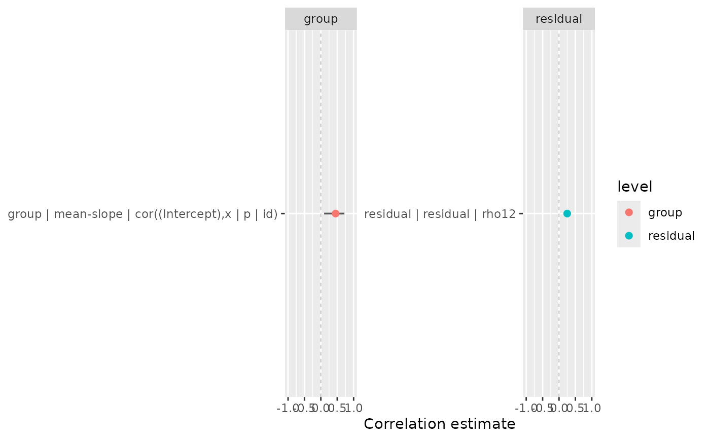
plot_corpairs() is a small ggplot2 consumer for tables returned by corpairs(). It does not compute correlation pairs, fit intervals, or choose a correlation layer. Build the table first with corpairs(), then pass that table to this helper.

Usage

plot_corpairs(
  data,
  colour = "level",
  facet = NULL,
  label = NULL,
  interval = TRUE,
  interval_style = c("eye", "line"),
  ...
)

Arguments

data

A data frame returned by corpairs(), or a compatible table with columns level, class, parameter, estimate, and modelled. conf.status and interval_source are optional for point-only tables, but finite intervals are drawn only when those columns mark a supported interval.

colour

Optional character scalar naming a column to map to colour. Use NULL to suppress colour mapping.

facet

Optional character scalar naming a column to facet by. Use NULL to suppress faceting.

label

Optional character scalar naming a column to use for y-axis row labels. Use this for publication figures where the full level | class | parameter label is too long. If NULL, labels are built from level, class, and parameter.

interval

Logical; draw finite conf.low/conf.high intervals when those columns are present.

interval_style

Character scalar. "eye" draws the default Confidence Eye region plus hollow point estimate. "line" draws conventional interval segments. Ignored when interval = FALSE.

...

Reserved for future options.

Value

A ggplot object.

Details

The helper draws one hollow point per correlation row. If the table contains finite conf.low and conf.high bounds plus interval provenance columns that describe a real interval, the default draws a pale Confidence Eye for those rows only, using a guarded Fisher-z/atanh correlation scale to shape the eye. The zero-correlation reference is dotted. Rows without supported bounds remain visible as point estimates and keep their display interval status attached to the plotted data. Set interval_style = "line" for a conventional CI-line variant.

Examples

pairs <- data.frame(
  level = c("residual", "group", "phylo", "group"),
  class = c("residual", "mean-slope", "structured", "scale-scale"),
  parameter = c(
    "rho12",
    "cor((Intercept),x | p | id)",
    "cor(mu1,mu2 | species)",
    "cor(sigma1,sigma2 | site)"
  ),
  label = c(
    "Residual\nrho12",
    "Group\nmean-slope cor",
    "Phylogenetic\nmu1-mu2",
    "Group\nsigma block"
  ),
  estimate = c(0.25, 0.45, -0.30, 0.12),
  modelled = c(FALSE, FALSE, FALSE, FALSE),
  conf.low = c(0.05, 0.10, -0.55, -0.12),
  conf.high = c(0.43, 0.72, -0.08, 0.34),
  conf.status = rep("profile", 4),
  interval_source = rep("profile", 4)
)
if (requireNamespace("ggplot2", quietly = TRUE)) {
  pair_palette <- c(
    group = "#D55E00",
    phylo = "#009E73",
    residual = "#0072B2"
  )
  plot_corpairs(pairs, label = "label") +
    ggplot2::scale_colour_manual(values = pair_palette) +
    ggplot2::scale_fill_manual(values = pair_palette) +
    ggplot2::theme_minimal(base_size = 11) +
    ggplot2::theme(
      panel.grid.major.y = ggplot2::element_blank(),
      panel.grid.minor.y = ggplot2::element_blank()
    ) +
    ggplot2::guides(colour = "none")
}