Association between mixed outcome pairs

Use this page when you have two outcomes measured on the same individual, site, or sampling occasion, but the outcomes need different models. For example, you might record whether an individual bred (0 or 1) and how many offspring it produced (a count). The question is: after accounting for predictors such as habitat, do rows that do better than expected for one outcome also tend to do better than expected for the other?

The one-call tool on this page returns that association and its numerical diagnostics. For every admitted pair route it also provides two-stage Godambe standard errors and Wald confidence intervals for the association-link coefficients alpha when fit-specific diagnostics pass. This interval surface is beta and deliberately scoped; it is not a general bivariate-family interface. If both outcomes are Gaussian and you need a jointly fitted model, use biv_gaussian() and its residual correlation rho12 instead.

Behind the scenes, the tool fits each outcome model first, holds those fitted margins fixed, and estimates a latent-normal association called eta. You do not need to understand that machinery before deciding whether the question and data requirements below match your study.

The question in an ecological example

Suppose each individual has a breeding outcome (0 or 1) and an offspring count. Habitat may explain both outcomes. The question is not whether the raw zeroes and counts have a large Pearson correlation. It is:

After habitat has been accounted for in each outcome, do individuals that are more likely than expected to breed also tend to have more offspring than expected?

The answer is expressed on an unobserved common scale. A positive eta means that the same rows tend to be unexpectedly high for both fitted outcomes on that unobserved Gaussian scale. It does not mean that eta is an odds ratio, a logit coefficient, an observed-scale correlation, or native residual rho12.

One call, two stages

biv_associate() is a convenience wrapper. It makes the workflow one R call, but it is still a two-stage estimator: it fits the two margins, freezes their estimated parameters, and estimates only eta in stage 2. Changing the stage-2 association never refits the mean or scale parameters from either margin.

Start with the callable workflow; the diagram and equations below explain what that call does. Create one data frame containing both responses and every predictor, then remove incomplete rows once. A binary response must contain exactly one literal 0 or 1 per row.

set.seed(20260801)
n <- 160L
habitat_score <- seq(-1.5, 1.5, length.out = n)
shared_tendency <- rnorm(n)

paired_data <- data.frame(
  habitat_score = habitat_score,
  bred = rbinom(
    n,
    size = 1,
    prob = plogis(-0.3 + 0.25 * habitat_score + 0.7 * shared_tendency)
  ),
  offspring = rnbinom(
    n,
    mu = exp(0.7 + 0.2 * habitat_score + 0.6 * shared_tendency),
    size = 2
  )
)

assoc <- biv_associate(
  bf(mu = bred ~ habitat_score),
  bf(mu = offspring ~ habitat_score, sigma = ~ 1),
  family = list(binomial(), nbinom2()),
  data = paired_data,
  association = ~ 1
)

association(assoc)
#>          kernel                  estimand       eta   status boundary
#> 1 latent_normal latent-normal association 0.3499604 interior    FALSE
alpha_se <- sqrt(diag(vcov(assoc)))
#> Warning: Association uncertainty is experimental for this lower-information fit (n =
#> 160).
#> ℹ The original lower-information campaign had unavailable intervals in some
#>   cells; this fit passed its numerical covariance diagnostics.
#> ℹ The retained high-information calibration campaign used n = 480 or 960.
alpha_se
#>     alpha 
#> 0.1084084
suppressWarnings(confint(assoc))
#>           2.5 %    97.5 %
#> alpha 0.1529225 0.5778756
suppressWarnings(confint(assoc, type = "eta"))
#>         2.5 %    97.5 %
#> eta 0.1517414 0.5211191

The first uncertainty request prints the experimental interval warning once for this lower-information example. The later calls suppress the duplicate warning so the rendered page keeps the coefficient and eta intervals readable.

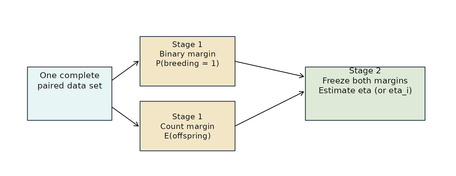
The frozen-margin workflow. The two response models are fitted first on the same complete rows. Their fitted probabilities or distributions are held fixed while stage 2 estimates a latent-normal association, eta. For every admitted route, the public Godambe covariance propagates uncertainty from both fitted margins into alpha-scale Wald intervals when fit-specific diagnostics pass.

In symbols, stage 1 produces two fitted marginal parameter sets, $\widehat\theta_1$ and $\widehat\theta_2$. Stage 2 estimates

$$\widehat\beta_A = \arg\max_{\beta_A} \sum_i \log f_{\eta_i}(y_{1i}, y_{2i} \mid \widehat\theta_1, \widehat\theta_2), \qquad a_i=X_{A,i}\beta_A,\quad \eta_i = \tanh(a_i).$$

For the usual constant association, $X_A=1$, so every row has the same eta. The beta Bernoulli x ordinary-NB2 slope route uses $X_{A,i}=(1,x_i)$. In computation, drmTMB keeps eta infinitesimally inside -1 and 1, because exact endpoints make the latent-normal probability calculation unstable. This is a plug-in association criterion, not a joint maximum-likelihood fit. The stage-2 Hessian alone therefore cannot give an ordinary valid standard error because it treats stage-1 uncertainty as fixed. Every admitted pair route instead uses the stacked stage-1 and stage-2 estimating equations to form a Godambe covariance for its alpha coefficients. This establishes interval feasibility. The Bernoulli x ordinary-NB2 intercept route additionally has retained coverage calibration.

Writing the full staged parameter as $q=(\theta_B^\top,\theta_N^\top,\alpha)^\top$ and its per-row stacked score as $U_i(q)$, drmTMB computes

$$H=-\frac{1}{n}\sum_i\frac{\partial U_i}{\partial q^\top},\qquad J=\frac{1}{n}\sum_i U_iU_i^\top,\qquad \widehat{\operatorname{Var}}(\widehat q)=\frac{1}{n}H^{-1}JH^{-\top}.$$

vcov(assoc) returns the alpha block of this matrix and confint(assoc) forms Wald intervals from that block. Thus the equations, R method, and reported target all use the same unbounded association-link scale.

For a design row $x_i^\top$, the bounded association is $\eta_i=0.999999\tanh(x_i^\top\alpha)$. predict() obtains its standard error from the delta method and obtains its confidence limits by transforming the link-scale Wald endpoints. The transformed interval therefore remains inside the valid eta range.

What a binary outcome contributes

A binary observation has no ordinary numeric residual. If the breeding margin predicts a probability $p_i = 0.80$, we observe only whether breeding happened, not how far above or below its predicted tendency the individual lay.

The association calculation uses an auxiliary latent variable $U_{Bi}$:

$$U_{Bi} \sim N(0, 1), \qquad B_i = 1\{U_{Bi} > \Phi^{-1}(1 - p_i)\}.$$

This threshold gives $P(B_i = 1) = p_i$. The latent variable is not an individual measurement and should not be reported as an individual binary residual. For a Gaussian outcome, the corresponding latent quantity is its standardized residual $(Y_i - \mu_i)/\sigma_i$. eta describes the correlation between these latent quantities after the margins are frozen.

Reviewed pair classes

A binary response in a reviewed pair cannot be a proportion, a cbind(successes, failures) response, or a binomial count with multiple trials.

The current reviewed classes are Gaussian x literal-Bernoulli, Gaussian x ordinary-NB2, literal-Bernoulli x literal-Bernoulli, literal-Bernoulli x ordinary-NB2, and ordinary-NB2 x ordinary-NB2. The last two show why “cross-family” is only a historical label for this page: the same frozen-margin machinery also has two reviewed same-family discrete classes.

association(assoc) returns eta unless the numerical diagnostic is boundary_unresolved; a near_boundary status remains flagged. For the example, a positive value says that a greater latent tendency to breed is associated with a greater latent tendency for offspring after habitat and season have been accounted for. It is not a raw-data correlation.

Standard error and confidence interval

For every admitted pair class, vcov(assoc) returns a named covariance matrix for the unbounded association-link coefficients alpha and confint(assoc) returns the corresponding alpha-scale Wald intervals when fit-specific diagnostics pass. These methods propagate fitted-margin uncertainty through a two-stage Godambe sandwich; they do not use the conditional stage-2 Hessian.

Keep the reported scale visible. The coefficient interval and the derived eta interval answer related but different questions:

association(assoc)       # bounded latent-normal eta point estimate
sqrt(diag(vcov(assoc)))  # Godambe SE for alpha
confint(assoc)           # Wald interval for alpha
confint(assoc, type = "eta") # transformed interval for constant eta

All admitted routes are interval-feasible. Those without route-specific coverage calibration warn that their intervals are experimental. The intercept-only Bernoulli x ordinary-NB2 route is inference-ready with caveats. In its retained high-information campaign (n = 480 or 960), all 16 cells passed the predeclared bias, availability, SE-calibration, and 95% coverage gates; cell coverage ranged from 0.935 to 0.957. The earlier lower-information campaign (n = 120 or 240) failed five primary coverage cells because some intervals were unavailable. Accordingly, lower-information fits are not blocked: a numerically valid covariance is returned with a warning, while an unstable or boundary result returns an informative error rather than a placeholder interval.

That coverage evidence does not transfer automatically to association slopes, other family pairs, random effects, incomplete pairs, weights, offsets, or REML. The eta transformation inherits the underlying alpha method’s tier; it does not create a new coverage claim. Association slopes and other family pairs remain interval-feasible, while the remaining features stay outside the current interval surface.

When the estimate or interval is withheld

For pairs with two discrete outcomes, the calculation evaluates a bivariate normal probability region that corresponds to the observed outcome pair. Some extreme tail regions can be numerically unresolved. In that case drmTMB withholds eta and its interval rather than clipping a probability or reporting a repaired estimate.

if (identical(assoc$status, "boundary_unresolved")) {
  assoc$diagnostics
  # Report that no association estimate was returned. Do not clip or repair it.
}

Inspect the diagnostics and report that no association estimate was available. Use Errors, warnings, and convergence for the next checks; do not convert an unresolved tail calculation into a scientific conclusion.

Can the association itself be modelled?

Usually start with association = ~ 1: it estimates one common eta after the predictors in the two margins have been accounted for. In the beta literal-Bernoulli x ordinary-NB2 route only, you can instead use an intercept-bearing fixed-effect formula with multiple predictors, factors, interactions, or explicit transformations. For example, suppose habitat_score is a numeric environmental gradient:

assoc_by_habitat <- biv_associate(
  bf(mu = bred ~ habitat_score),
  bf(mu = offspring ~ habitat_score, sigma = ~ season),
  family = list(binomial(), nbinom2()),
  data = paired_data,
  association = ~ habitat_score
)

association(assoc_by_habitat)
association(assoc_by_habitat, type = "fitted")

new_habitats <- data.frame(habitat_score = c(-1, 0, 1))
predict(
  assoc_by_habitat,
  newdata = new_habitats,
  type = "eta",
  se.fit = TRUE,
  interval = "confidence"
)

This simple formula fits $a_i=\beta_0+\beta_1\,\texttt{habitat_score}_i$ and converts it to a row-specific latent association $\eta_i=\tanh(a_i)$. association() first returns the two coefficients on the association-link scale; type = "fitted" returns the corresponding eta_i values for the rows used to fit the margins. vcov() and confint() also return the two-by- two alpha covariance and coefficient intervals for this slope model. They are interval-feasible and explicitly uncalibrated for coverage.

The same route accepts formulas such as ~ habitat_score + season, ~ habitat, or ~ habitat_score * habitat, and predict() evaluates the fitted association link or bounded eta at compatible newdata. Its standard errors are pointwise delta-method results, and its eta confidence limits are transformed link-scale Wald intervals. They are not simultaneous bands.

This is similar in spirit to allowing a predictor for a residual rho12, but it is not the same model or parameter. rho12 belongs to a direct joint likelihood, whereas this beta route freezes two separately fitted margins before estimating its association link. Random effects, offsets, missing association predictors, aliased design columns, dot expansion, and association regressions for the other pair classes remain unsupported.

Question	Current beta answer
Does habitat predict breeding?	Put habitat in the binary margin.
Does season predict offspring variation?	Put season in the count sigma margin.
Is there one remaining association after those effects?	Estimate association = ~ 1.
Does association change along one numeric habitat score?	For beta Bernoulli x ordinary-NB2 only, use association = ~ habitat_score.
Does association change among habitat categories or with several predictors?	For beta Bernoulli x ordinary-NB2 only, use an intercept-bearing fixed-effect formula and preserve its fitted factor levels for prediction.

How this differs from rho12

rho12 belongs to a direct joint likelihood. In biv_gaussian() it is a Gaussian residual correlation; in biv_lognormal() it is a log-response residual correlation. eta is neither of those. It is a latent-normal association obtained after separate margins have been fitted and frozen. The new beta association slope changes the latent eta_i, not a direct rho12.

Use Changing residual coupling with rho12 for the released Gaussian joint model. Use Bivariate non-Gaussian models to choose between an exact same-family joint model and this staged association route.