
Bivariate non-Gaussian models: choose a joint or staged association
Source:vignettes/bivariate-nongaussian.Rmd
bivariate-nongaussian.RmdWith two non-Gaussian outcomes, first decide what kind of association answers the scientific question. A direct joint likelihood estimates both outcomes and their residual association together. A frozen-margin association first fits the two outcomes separately and then estimates a latent-normal association while holding the fitted margins fixed. These are different estimands.
This article helps you choose a route for two outcomes measured on
the same rows. For reviewed mixed outcome pairs, the staged route
reports alpha-scale Godambe standard errors and Wald intervals. The
Bernoulli x ordinary-NB2 intercept route has been studied for interval
coverage, but coverage is not yet established for the other admitted
pairs. Random effects and a generic family-pair interface remain outside
this staged route. The direct lognormal route also provides uncertainty
methods for a constant rho12, but a finite interval alone
does not establish a general non-Gaussian result. For a released direct
Gaussian joint model, use biv_gaussian() and Changing residual coupling with
rho12.
Start by choosing the association scale
| Your paired outcomes | Route | What the association means |
|---|---|---|
| Two Gaussian traits | Direct biv_gaussian() model |
Gaussian residual rho12
|
| Two positive traits plausibly lognormal | Direct biv_lognormal() model |
Log-response residual rho12
|
| Two heavy-tailed real-valued traits | Direct biv_student() model |
Shared-Student-t residual/scatter rho12
|
| A reviewed mixed or discrete pair |
biv_associate() staged route |
Latent-normal copula eta after frozen margins; an
intercept-bearing fixed-effect association formula is interval-feasible
for Bernoulli x NB2 |
Neither rho12 nor eta is automatically the
Pearson correlation of the two raw response columns. The scale is part
of the scientific interpretation, not just a computational detail.
Direct joint model: two positive traits
For two positive lognormal outcomes, the model is joint on the log-response scale:
Here rho12 is the correlation of the two log-response
residuals. A positive value means that units above their fitted
log-response expectation on one trait also tend to be above it on the
other. It is not automatically the correlation of the two traits on
their original scale.
Real example: penguin size after measured composition differences
The openly licensed palmerpenguins data set records body
size in three Palmer Archipelago penguin species. It is distributed
under CC0 and collates data from the Palmer Station LTER study (data policy;
Gorman et
al. 2014).
Our question is conditional: after allowing both margins to vary by species, sex, and centred year, do birds with longer-than-expected flippers also have greater-than-expected body mass? This is not a causal claim that flippers determine mass, nor a replacement for a raw scatterplot.
penguins <- subset(
  palmerpenguins::penguins,
  complete.cases(species, sex, year, flipper_length_mm, body_mass_g) &
    flipper_length_mm > 0 & body_mass_g > 0
)
penguins$year_c <- penguins$year - mean(penguins$year)
nrow(penguins)
#> [1] 333
plot(
  log(body_mass_g) ~ log(flipper_length_mm), data = penguins,
  pch = 16, col = grDevices::adjustcolor("#087f8c", alpha.f = 0.45),
  xlab = "log flipper length (mm)", ylab = "log body mass (g)"
)
abline(stats::lm(log(body_mass_g) ~ log(flipper_length_mm), data = penguins),
  col = "#14344a", lwd = 2
)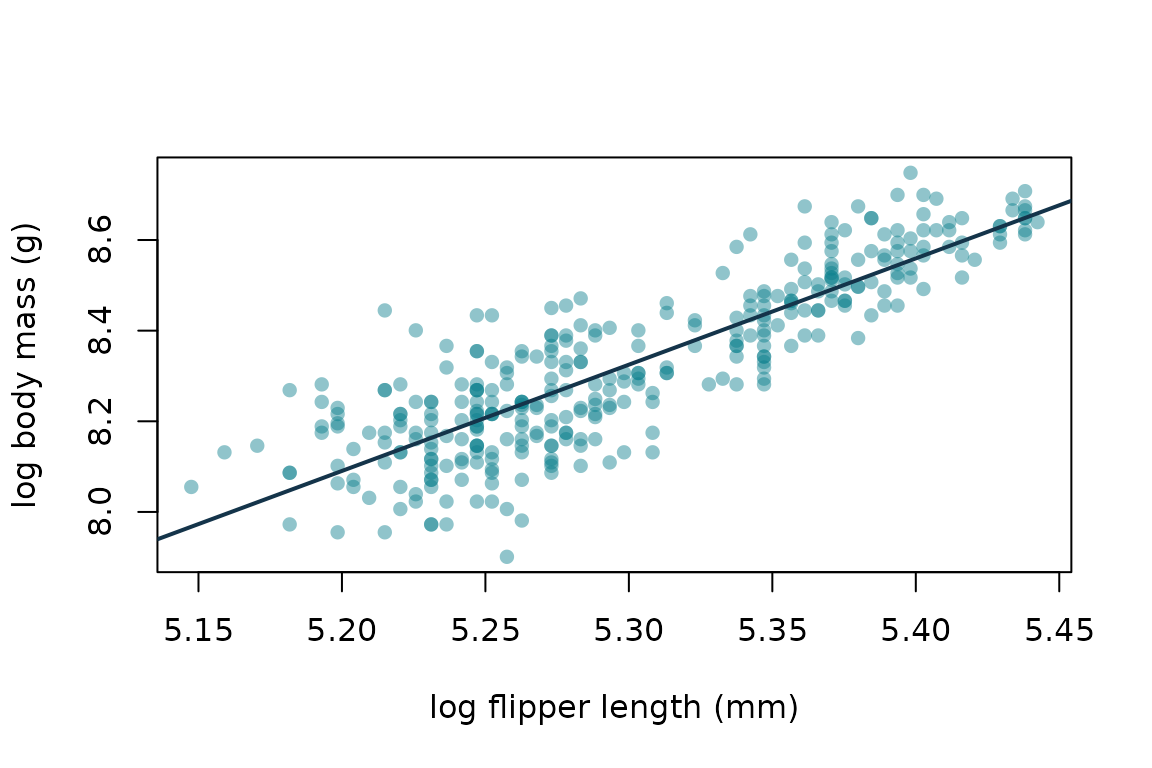
Raw log-scale flipper length and body mass for analysed complete rows. This descriptive relationship is not the fitted residual association.
fit_log <- drmTMB::drmTMB(
drmTMB::bf(mu1 = flipper_length_mm ~ species + sex + year_c,
mu2 = body_mass_g ~ species + sex + year_c,
sigma1 = ~ 1, sigma2 = ~ 1, rho12 = ~ 1),
family = drmTMB::biv_lognormal(), data = penguins
)
drmTMB::rho12(fit_log)[1]
#> [1] 0.3583776
drmTMB::check_drm(fit_log)
#> <drm_check: 18 checks>
#> check status
#> optimizer_convergence ok
#> convergence_status ok
#> optimizer_budget ok
#> finite_objective ok
#> logsigma_clamp_active ok
#> fixed_gradient ok
#> sdreport_status ok
#> hessian_positive_definite ok
#> hessian_conditioning ok
#> standard_errors_finite ok
#> standard_errors_inflated ok
#> mle_existence ok
#> observations_per_parameter ok
#> fixed_effect_collinearity ok
#> dropped_rows ok
#> positive_scale ok
#> rho12_boundary ok
#> fixed_effect_design_size ok
#> value
#> 0
#> converged
#> iterations=13; function=30; gradient=13
#> 3403.
#> <NA>
#> max=0.0000000001547; component=beta_mu1[1]
#> ok
#> TRUE
#> min_eig=298.3; cond=2683.
#> range=[0.001821,0.05480]
#> n_inflated=0; max_se=0.05480; reference_median=0.007649
#> finite
#> n_obs=333; n_par=13; ratio=25.62
#> max_abs_r=0.3777
#> nobs=333; dropped=0
#> min=0.02695
#> 0.3584
#> total_mb=0.1401; max_cols=5; largest=mu1; largest_class=matrix; largest_density=0.6132
#> message
#> nlminb convergence code is 0.
#> Optimizer convergence and uncertainty diagnostics are consistent with a proper interior optimum.
#> Optimizer evaluation counts recorded; no eval.max or iter.max control was supplied.
#> Objective and log-likelihood are finite.
#> The log(sigma) clamp is not active at the optimum.
#> Maximum absolute fixed gradient is <= 0.001; largest component is beta_mu1[1].
#> TMB::sdreport() completed successfully.
#> sdreport reports a positive-definite Hessian.
#> Minimum eigenvalue and condition number of TMB's sdreport() fixed-effect covariance (sdr$cov.fixed), inverted. These are a genuinely different read of the fit's conditioning than TMB's internal pdHess flag -- comparable across fits, not claimed to be numerically identical to any raw TMB gradient or Hessian quantity. This fit's Hessian conditioning is within the requested threshold.
#> All fixed-effect standard errors are finite.
#> No fixed-effect standard error is inflated relative to the others.
#> The screened fixed-effect geometry is consistent with a finite maximum-likelihood estimate.
#> Observations per estimated parameter are at or above the small-samplenote threshold (10).
#> No fixed-effect design column pair exceeds the collinearity note threshold.
#> No rows were dropped by model-frame or known-covariance filtering.
#> All fitted scale values are finite and positive.
#> All fitted residual correlations have absolute value <= 0.98.
#> Dense fixed-effect design matrices are modest for this fit.
# All three target the log-residual rho12, not a raw-scale correlation.
ci_wald <- confint(fit_log, parm = "rho12", method = "wald")
ci_profile <- confint(
fit_log, parm = "rho12", method = "profile", profile_engine = "endpoint"
)
ci_bootstrap <- confint(
fit_log, parm = "rho12", method = "bootstrap", R = 99, seed = 20260724
)
interval_row <- function(x, label) {
data.frame(
label = label,
estimate = unname(drmTMB::rho12(fit_log)[1]),
lower = x$lower,
upper = x$upper,
status = x$conf.status,
note = x$profile.message,
stringsAsFactors = FALSE
)
}
intervals <- rbind(
interval_row(ci_wald, "Wald"),
interval_row(ci_profile, "Profile"),
interval_row(
ci_bootstrap,
sprintf(
"Bootstrap (%d/%d retained)",
ci_bootstrap$bootstrap.n,
ci_bootstrap$bootstrap.n + ci_bootstrap$bootstrap.failed
)
)
)
bootstrap_total <- ci_bootstrap$bootstrap.n + ci_bootstrap$bootstrap.failed
cat(sprintf(
"Bootstrap diagnostic: %d/%d full refits retained. Failed refits remain a diagnostic, not hidden precision.\n",
ci_bootstrap$bootstrap.n, bootstrap_total
))
#> Bootstrap diagnostic: 99/99 full refits retained. Failed refits remain a diagnostic, not hidden precision.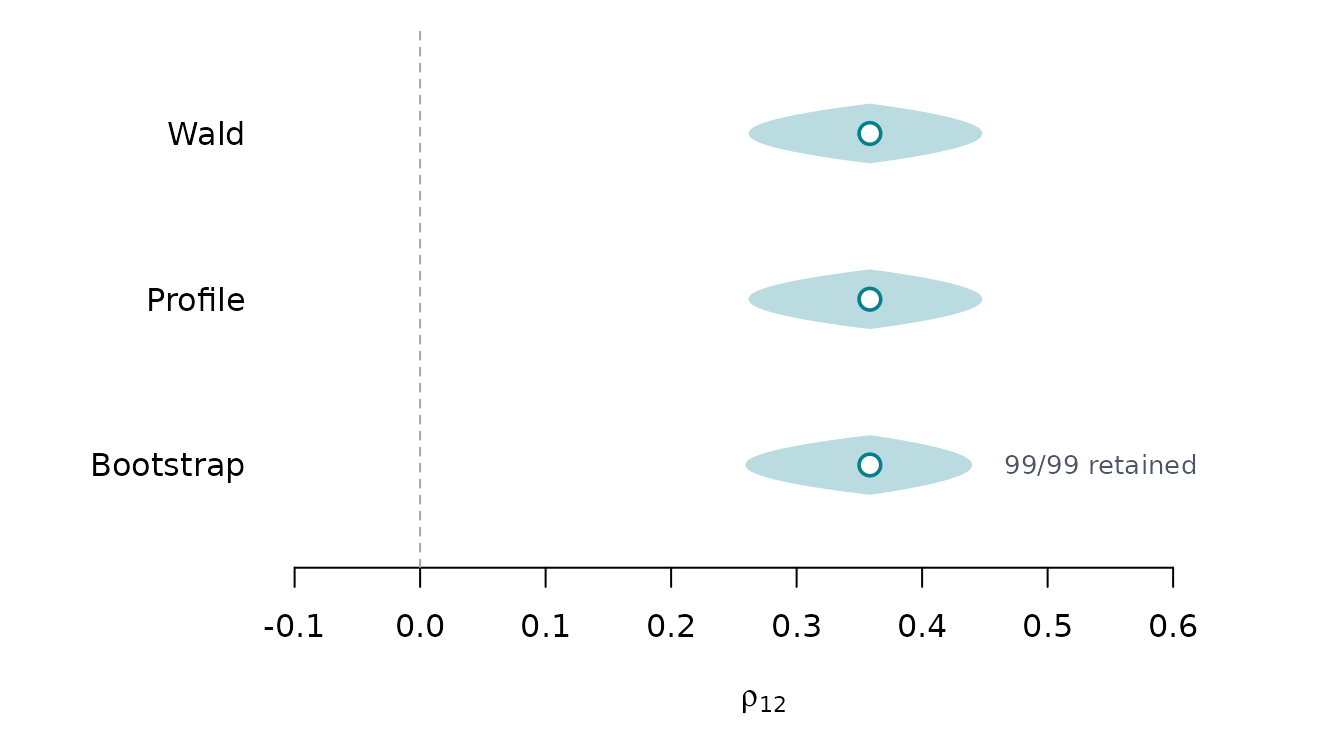
Reported 95% confidence intervals for the fitted direct log-residual association in the penguin model. Each eye spans the reported interval and is centred on its estimate; the taper is a visual interval cue, not a likelihood, sampling density, or posterior distribution. The retained bootstrap count is a diagnostic, not hidden precision.
fitted(fit_log) returns arithmetic marginal means on the
original response scale. The mu1 and mu2
predictors remain log-scale locations. These direct models estimate the
two margins and rho12 together; they are not staged
frozen-margin fits. Wald is a fast link-scale approximation; profile
likelihood checks the exact likelihood geometry; the bootstrap refits
both margins and rho12. Inspect
check_drm(fit_log) and bootstrap diagnostics, especially
near
.
In this data set, do not hide failed bootstrap refits: the printed
bootstrap.n and bootstrap.failed fields are
part of the result. The external data example illustrates interpretation
and diagnostics; it does not itself establish coverage calibration or
prove lognormal adequacy. Inspect residual diagnostics and compare
scientifically defensible alternatives before reporting a substantive
association.
If a fit, covariance, or interval is withheld, follow Errors, warnings, and convergence rather than repairing, clipping, or hiding the diagnostic result.
Direct joint model: two heavy-tailed traits
For two real-valued traits with occasional extreme observations, the
bivariate Student-t model uses a shared degrees-of-freedom parameter,
nu:
fit_t <- drmTMB(
  bf(mu1 = activity ~ habitat, mu2 = boldness ~ habitat,
     sigma1 = ~ 1, sigma2 = ~ 1, nu = ~ 1, rho12 = ~ 1),
  family = biv_student(), data = behaviour
)

rho12(fit_t)
sigma1 and sigma2 are Student-t scales, not
necessarily marginal standard deviations. The model has one shared
nu, which controls tail heaviness. At a finite
nu, rho12 = 0 means zero residual correlation,
but not necessarily complete independence because the two outcomes share
the same row-level heavy-tail mechanism.
Staged association: different kinds of outcome
If one response is binary and the other is a count, there is no
shared direct Gaussian residual scale. The frozen-margin route instead
fits a binary probability model and a count model, then estimates
latent-normal eta from their fitted distributions.
paired_data <- na.omit(data.frame(
  bred, offspring, habitat, habitat_score, season
))

assoc <- biv_associate(
  bf(mu = bred ~ habitat),
  bf(mu = offspring ~ habitat, sigma = ~ season),
  family = list(binomial(), nbinom2()),
  data = paired_data,
  association = ~ 1
)

association(assoc)
vcov(assoc)
confint(assoc)
confint(assoc, type = "eta")
This is one convenient R call, but not one jointly fitted model.
biv_associate() fits the two margins, freezes them, and
estimates only eta. The reported value is a latent-normal
copula correlation conditional on those fitted margins. It is not
rho12, a logit coefficient, an odds ratio, or an
observed-scale correlation. For every admitted association route,
vcov() and plain confint() report two-stage
Godambe uncertainty for the unbounded association-link coefficients
alpha whenever the fit-specific covariance diagnostics
pass. confint(assoc, type = "eta") transforms the constant-
association interval to bounded eta, while predict()
supplies delta-method eta standard errors and pointwise transformed
intervals.
For a binary response, the model observes whether a hidden tendency crossed a threshold. It does not observe an ordinary numeric residual. Read Frozen-margin association for mixed outcome pairs for the binary-threshold explanation, the reviewed pair classes, and the rule for withheld estimates.
For the literal-Bernoulli x ordinary-NB2 beta route, an
intercept-bearing fixed-effect formula such as
association = ~ x, ~ habitat, or
~ x * habitat can model a row-specific latent-normal
eta_i after both margins have been fitted and frozen.
Multiple predictors, factors, interactions, and explicit transformations
use the ordinary fixed-effect model matrix. See Association between mixed outcome pairs for
the exact syntax, output, and limits.
What is currently outside these routes
The direct same-family first slices keep sigma1,
sigma2, rho12, and nu constant
across rows. The staged route usually keeps eta constant;
its beta exception is an intercept-bearing fixed-effect association
formula for literal-Bernoulli x ordinary-NB2. Its reviewed fixed-effect
margins may include their explicitly supported covariates before they
are frozen. Neither route currently adds random effects or missing-data
support, and the staged formula rejects offsets, missing predictors,
aliased columns, dot expansion, and random effects. Other pair classes
remain intercept-only. Neither route is a general non-Gaussian bivariate
claim. The staged route’s alpha-scale standard errors and Wald intervals
are interval-feasible for every admitted pair class and for the
Bernoulli x ordinary-NB2 association-regression formula. Routes without
coverage has not been established, the fit warns before reporting an
interval. Eta uncertainty has the same limitation; simultaneous eta
bands and profiles remain unavailable. The direct lognormal
constant-rho12 profile, Wald, and bootstrap methods have
been checked only for a fixed-effect data-generating setting. They do
not validate the staged route or a general non-Gaussian association
claim. Choose the route whose stated association scale matches the
biological question, and treat every boundary as part of the model
definition. For the exact admitted mixed pairs and their output,
continue to Association between mixed
outcome pairs.
Working in Julia? The DRModels.jl
companion page mirrors this article with Julia syntax and states
which parts DRModels.jl supports today. DRModels.jl is a separate
package with its own fitting and inference routes; Julia is optional for
drmTMB users.