
Function map and cheat sheet
Source:vignettes/articles/function-map-cheatsheet.Rmd
function-map-cheatsheet.RmdUse this guide when drmTMB is installed and you know the
scientific task you want to do next, but not which function starts it.
For installation and a guided first fit, read the fuller package introduction. If you already know the
syntax and need to verify support, go directly to What can I fit today?.
This page is a navigation aid, not a claim that every displayed function, family, structured effect, or interval route is suitable for every model.
drmTMB can model location (a family-specific centre or
location parameter; for Gaussian models it is the expected response),
scale (residual variability), shape (distribution features beyond
location and scale), and coscale, meaning residual correlation such as
rho12 between two responses. Not every family exposes every
parameter, and a location parameter need not be the unconditional
response mean.
Find the next step
The ordinary route is Specify model → Fit → Check fit
health. After checking the fit, choose the branch that answers
the scientific question: interpret parameters, predict and assess, or
quantify uncertainty and simulate. If the fit is not healthy, revise the
specification and fit again. Structured terms such as
phylo(), spatial(), and relmat()
belong in the model specification; they are not a later analysis stage.
The gaussian() and nbinom2() labels in the
first box are examples of family constructors, not an exhaustive family
list.
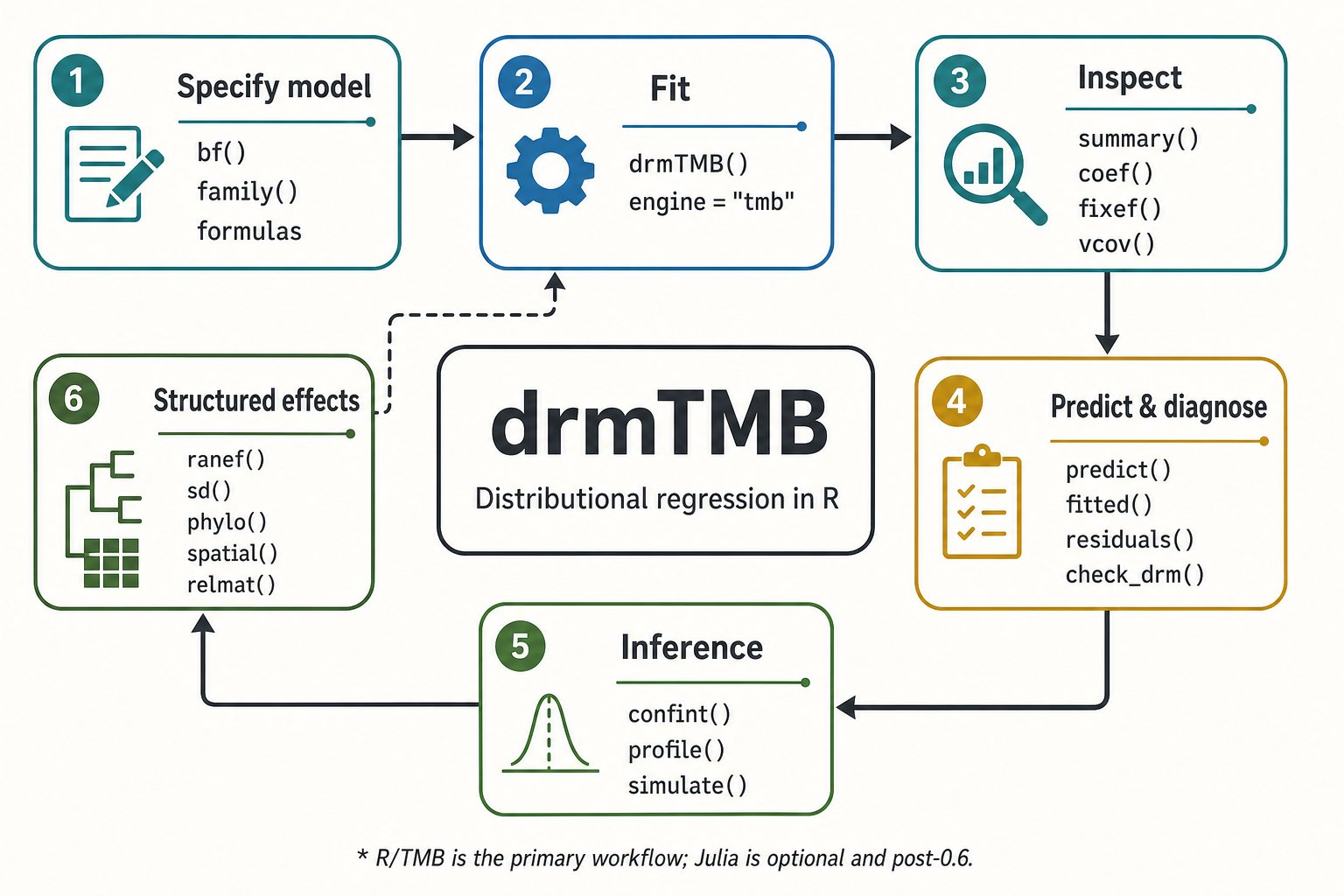
Open the full-size function map when reading on a small screen.
This HTML article is the accessible text alternative. The PDFs are untagged print companions; screen-reader users should use the route table and linked function descriptions on this page.
Typical route: Specify → Fit → Check. Interpretation, prediction, assessment, uncertainty, and simulation are conditional next tasks rather than compulsory stages.
The Predict & assess branch checks fitted-response and fixed-effect distributional form. It does not by itself establish adequacy of every random or structured component; follow Distributional outputs and adequacy for that boundary.
Choose a route
| Goal | Start with | Read next |
|---|---|---|
| Learn the model grammar and fit a first model |
bf(), a family object, drmTMB()
|
Full package introduction |
| Check numerical fit health before interpreting |
check_drm(), summary()
|
Model workflow |
| Resolve an error, warning, or unstable fit |
check_drm(), the original warning, and the fitted
object |
Errors, warnings, and convergence |
| Extract a parameter or make a prediction table |
coef(), fixef(),
predict_parameters()
|
Distributional outputs and adequacy |
| Study latent-normal association for a paired-outcome class listed in the association guide |
biv_associate(), association(),
vcov(), confint()
|
Association between outcome pairs |
| Work with repeated, related, or spatially structured data |
bf() with phylo(), spatial(),
or relmat(); then ranef()
|
Structural dependence overview |
| Request an interval or profile a target |
confint(), profile_targets(),
profile()
|
Checking and using fitted models |
| Fit when some values are missing |
miss_control(), mi(),
imputed()
|
Handling missing data |
| Ask what a fitted model’s objective is at some other parameter point, without refitting |
objective_at(),
drm_control(start = ...)
|
Checking and using fitted models |
| Record which build produced a result, when the version number cannot tell two builds apart | drm_provenance() |
Errors, warnings, and convergence |
| Confirm an unfamiliar route is supported | the model and capability guides | What can I fit today? |
The shortest useful workflow
Suppose an ecologist asks whether an environmental gradient changes
both mean growth and its predictability. For a continuous response,
write one formula for location mu and one for residual
scale sigma, then check the fit before interpreting it.
set.seed(20260721)
n <- 80
x <- rnorm(n)
dat <- data.frame(
y = 0.4 + 0.7 * x + rnorm(n, sd = exp(-0.3 + 0.2 * x)),
x = x
)
fit <- drmTMB(
bf(y ~ x, sigma ~ x),
family = gaussian(),
data = dat
)
check_drm(fit)
#> <drm_check: 15 checks>
#> ok: 15; notes: 0; warnings: 0; errors: 0
#> check status
#> optimizer_convergence ok
#> convergence_status ok
#> optimizer_budget ok
#> finite_objective ok
#> logsigma_clamp_active ok
#> fixed_gradient ok
#> sdreport_status ok
#> hessian_positive_definite ok
#> hessian_conditioning ok
#> standard_errors_finite ok
#> standard_errors_inflated ok
#> observations_per_parameter ok
#> dropped_rows ok
#> positive_scale ok
#> fixed_effect_design_size ok
#> value
#> 0
#> converged
#> iterations=11; function=21; gradient=12
#> 91.76
#> <NA>
#> max=0.0000000006002; component=beta_sigma[1]
#> ok
#> TRUE
#> min_eig=97.13; cond=1.881
#> range=[0.07841,0.09395]
#> n_inflated=0; max_se=0.09395; reference_median=0.08237
#> n_obs=80; n_par=4; ratio=20.00
#> nobs=80; dropped=0
#> min=0.5884
#> total_mb=0.01372; max_cols=2; largest=mu; largest_class=matrix; largest_density=1.000
#> message
#> nlminb convergence code is 0.
#> Optimizer convergence and uncertainty diagnostics are consistent with a proper interior optimum.
#> Optimizer evaluation counts recorded; no eval.max or iter.max control was supplied.
#> Objective and log-likelihood are finite.
#> The log(sigma) clamp is not active at the optimum.
#> Maximum absolute fixed gradient is <= 0.001; largest component is beta_sigma[1].
#> TMB::sdreport() completed successfully.
#> sdreport reports a positive-definite Hessian.
#> Minimum eigenvalue and condition number of TMB's sdreport() fixed-effect covariance (sdr$cov.fixed), inverted. These are a genuinely different read of the fit's conditioning than TMB's internal pdHess flag -- comparable across fits, not claimed to be numerically identical to any raw TMB gradient or Hessian quantity. This fit's Hessian conditioning is within the requested threshold.
#> All fixed-effect standard errors are finite.
#> No fixed-effect standard error is inflated relative to the others.
#> Observations per estimated parameter are at or above the small-samplenote threshold (10).
#> No rows were dropped by model-frame or known-covariance filtering.
#> All fitted scale values are finite and positive.
#> Dense fixed-effect design matrices are modest for this fit.
coef(fit, dpar = "mu")
#> (Intercept) x
#> 0.4806753 0.6758442
coef(fit, dpar = "sigma")
#> (Intercept) x
#> -0.2831455 0.1618192Here mu is expected growth and sigma is
residual SD. The sigma coefficients use a log-SD link:
exponentiating the slope gives the residual-SD ratio per one-unit
increase in x. Keep this residual scale separate from the
SD of a group-level random effect.
Make response-scale predictions on an explicit grid:
coef(fit, dpar = "mu")
#> (Intercept)           x
#>   0.4806753   0.6758442
coef(fit, dpar = "sigma")
#> (Intercept)           x
#>  -0.2831455   0.1618192

grid <- data.frame(x = c(-1, 0, 1))
predict_parameters(
  fit,
  newdata = grid,
  dpar = c("mu", "sigma"),
  conf.int = TRUE
)
#>   row row_label  dpar            component     type   estimate  std.error
#> 1   1         1    mu             location response -0.1951689 0.11176178
#> 2   2         2    mu             location response  0.4806753 0.08550270
#> 3   3         3    mu             location response  1.1565195 0.14065994
#> 4   1         1 sigma distributional-scale response  0.6408469 0.07385666
#> 5   2         2 sigma distributional-scale response  0.7534102 0.05970367
#> 6   3         3 sigma distributional-scale response  0.8857448 0.09528558
#>     conf.low  conf.high conf.level conf.status interval_source  x
#> 1 -0.4142180 0.02388017       0.95        wald            wald -1
#> 2  0.3130931 0.64825750       0.95        wald            wald  0
#> 3  0.8808311 1.43220789       0.95        wald            wald  1
#> 4  0.5112750 0.80325607       0.95        wald            wald -1
#> 5  0.6450277 0.88000387       0.95        wald            wald  0
#> 6  0.7173632 1.09364949       0.95        wald            wald  1
The prediction table records interval provenance in
conf.status and interval_source. If
check_drm() reports a warning or error, or an interval
status is unavailable, follow Errors,
warnings, and convergence before reporting the result. A
fixed-effect Wald interval does not establish calibrated coverage for a
random-effect SD.
If fitting stops before an object is returned, read the original
error and confirm the exact family-component combination in What can I fit today?. If a fit object is
returned, run check_drm(fit), address the flagged
optimizer, gradient, Hessian, or design problem, then refit and rerun
the check before interpreting.
Keep the boundaries visible
drmTMB() is the primary R workflow shown here. Julia
fitting remains future/deferred work; the current Julia methods provide
compatibility for legacy Julia-engine objects and are not a route for a
new analysis.
This page chooses a route; it does not establish a claim tier. Before a substantive analysis, confirm the exact family, model component, and inference boundary in What can I fit today? and What can I trust?. If the exact combination is absent or marked planned or diagnostic-only, do not treat a successful fit as supported inference; choose an implemented route or report the limitation.