Structural dependence details • drmTMB

This page assumes you have already used the structural-dependence overview or one of the worked tutorials (animal-models, phylogenetic-models, spatial-models, relmat-known-matrices) to choose a route; it collects the current fitted ladder across all of them in one place. Structural dependence means a random effect has a known dependence structure instead of independent group levels. Read the grammar in biological order: animal models for pedigree or additive relatedness, phylogenetic models for tree-structured relatedness, spatial models for coordinate or mesh structure, combined phylogenetic-plus-spatial models when both sources matter, and relmat() for other known relatedness or precision matrices.

The current fitted drmTMB paths are a subset of that ladder. For Gaussian models, phylo(), coordinate spatial(), animal(), and relmat() each fit one univariate mu intercept and one numeric mu slope. These one-slope paths estimate independent structured intercept and slope fields with separate SDs. Those Gaussian mu terms do not themselves establish multiple or labelled slopes, intercept-slope correlations, or structured residual rho12. Separate exact q1 sigma and non-Gaussian gates are fitted for the providers and families named in the route table below. A first bivariate path also fits matching intercept-only phylo() terms in mu1 and mu2, estimating the two phylogenetic location SDs and their mean-mean correlation. Matching labelled phylo() terms across mu1, mu2, sigma1, and sigma2 now fit the first constant bivariate phylogenetic location-scale block. The first predictor-dependent phylogenetic correlation regression is also fitted for the q=2 mu1-mu2 location-location row. The first coordinate-based spatial paths, spatial(1 | site, coords = coords) and spatial(1 + x | site, coords = coords), are fitted for univariate Gaussian location models. Matching labelled spatial(1 | p | site, coords = coords) terms in bivariate mu1 and mu2 fit the first coordinate-spatial mean-mean correlation, reported by corpairs(level = "spatial"); matching labelled spatial terms across mu1, mu2, sigma1, and sigma2 fit the first constant coordinate-spatial q=4 location-scale block. animal() and relmat() fit the same first Gaussian intercept and one-slope mu pattern when supplied with a pedigree, precomputed relationship, or precision matrix, such as animal(1 | id, pedigree = pedigree), animal(1 + x | id, Ainv = Ainv), or relmat(1 + x | id, Q = Q). Artifact routing is narrower than fitted syntax. The one-slope routes have manual Phase 18 artifact tasks named phylo_mu_slope, spatial_mu_slope, animal_mu_slope, and relmat_mu_slope. These tasks are opt-in, excluded from task = "all", and are not recovery, coverage, or power evidence. Mesh/SPDE spatial fields, combined phylogenetic-plus-spatial location models, additional multiple or labelled spatial-slope layouts outside the exact fitted ledger cells, spatial slope correlations, non-Gaussian spatial effects outside the exact ordinary Poisson/NB2 q1 spatial mu intercept-plus-one-slope, recovery-grade NB2 q1 spatial sigma, Student-t spatial mu, Poisson spatial zi, fixed-zi Poisson spatial mu, and fixed-zi NB2 spatial mu gates, and predictor-dependent spatial correlations remain planned extensions. The q1 spatial sigma one-slope route has point-fit/extractor evidence, but its interval gate remains blocked.

The scientific questions for the structural ladder are simple:

Do predictors explain trait means after accounting for resemblance among relatives, species, or nearby sites? Does a response still have smooth coordinate-based site deviations, or does a predictor’s slope vary smoothly across sites?

For animal models, individual or animal indexes rows in the data. A small id/dam/sire pedigree or a precomputed additive relatedness or inverse-relatedness matrix supplies expected genetic similarity. For phylogenetic models, species indexes the rows in the data and tree supplies the relatedness among those species. For spatial models, site indexes the rows in the data and coords supplies one coordinate pair per site, or one row per observation when coordinates are constant within site. In the fitted animal, phylogenetic, spatial, and relmat() paths, the structured term adds Gaussian coefficients to the location parameter mu. The intercept path adds an individual, species, site, or matrix-indexed deviation in mean response. The one-slope paths let the effect of one numeric predictor vary across the same structured levels.

Throughout this article, Normal(a, b) and MVN(a, B) use variance or covariance as the second argument.

In this article, a location parameter such as mu describes the expected trait value, a scale parameter such as sigma describes residual or random-effect variability, a shape parameter such as nu describes a family-specific feature such as tail weight or skewness, and a coscale parameter models residual correlation, such as bivariate rho12. Structured animal, phylogenetic, and spatial effects are not residual coscale terms unless the fitted model explicitly includes a residual rho12 formula.

Reader route: animal, phylo, spatial, phylo+spatial, relmat

Read this page as a five-step structural-dependence ladder. Step 1 asks whether individuals resemble each other because of pedigree or additive relatedness. Step 2 asks whether related species remain similar after fixed effects. Step 3 asks whether nearby sites remain similar after fixed effects. Step 4 asks whether both species relatedness and site coordinates are needed in the same model. Step 5 is the lower-level relmat() route for known dependence matrices that do not belong to the named animal, phylogenetic, or spatial routes. In the current package, Steps 1, 2, 3, and 5 have fitted Gaussian paths plus exact row-specific non-Gaussian gates; Step 4 is documented planned syntax.

For a one-response phylogenetic-plus-spatial endpoint such as heat_tolerance, the conceptual full model is:

$\begin{aligned} y_i &\sim \operatorname{Normal}(\mu_i, \sigma_i^2),\\ \mu_i &= \mathbf{x}_i^\top\boldsymbol{\beta}_{\mu} + a_{\mathrm{species}[i]} + s_{\mathrm{site}[i]},\\ \mathbf{a} &\sim \operatorname{MVN}(\mathbf{0}, \sigma^2_{\mathrm{phylo}}\mathbf{A}),\\ \mathbf{s} &\sim \operatorname{MVN}(\mathbf{0}, \sigma^2_{\mathrm{space}}\mathbf{M}),\\ \log(\sigma_i) &= \mathbf{z}_i^\top\boldsymbol{\beta}_{\sigma}. \end{aligned}$

Here $y_i$ is the observed trait, for example heat tolerance for individual or species-site observation $i$ . The vector $\mathbf{x}_i$ contains location predictors such as habitat temperature or body mass, and $\boldsymbol{\beta}_{\mu}$ are their average effects on the expected trait value. The term $a_{\mathrm{species}[i]}$ is the phylogenetic deviation for the species attached to observation $i$ , $\mathbf{A}$ is the phylogenetic covariance implied by the tree, and $\sigma_{\mathrm{phylo}}$ is the SD of tree-structured location deviations. The term $s_{\mathrm{site}[i]}$ is the spatial deviation for the sampling site, $\mathbf{M}$ is the coordinate-based spatial covariance, and $\sigma_{\mathrm{space}}$ is the SD of spatial location deviations. The vector $\mathbf{z}_i$ contains residual-scale predictors and $\boldsymbol{\beta}_{\sigma}$ are their effects on log residual SD.

The animal-model analogue replaces the species term with an individual additive effect, for example $\mathbf{g} \sim \operatorname{MVN}(\mathbf{0}, \sigma^2_{\mathrm{animal}}\mathbf{A}_{\mathrm{pedigree}})$ . That is the meaning of animal(1 | individual, pedigree = pedigree), animal(1 | individual, A = A), or animal(1 | individual, Ainv = Ainv). The pedigree route builds a dense additive relationship matrix for this first Gaussian location path; sparse large-pedigree precision construction remains planned.

Read the current route status this way:

Route	Current status	Use when	Syntax to read
1. Animal	Implemented for the documented Gaussian routes plus exact ordinary Poisson/NB2 q1 `mu` intercept-plus-one-slope, NB2 q1 `sigma`, and beta animal gates at their recorded tiers; sparse large-pedigree construction remains planned	Individuals have known additive relatedness from a pedigree or relationship matrix, and the biological question is an animal model or quantitative-genetic random effect.	`animal(1 \| individual, pedigree = pedigree)`, `animal(1 + x \| individual, Ainv = Ainv)`, or matching labelled Gaussian terms; consult the live ledger before using a non-Gaussian animal gate
2. Phylo	Implemented for the documented Gaussian routes plus exact ordinary Poisson/NB2 q1 `mu` intercept-plus-one-slope, NB2 q1 `sigma`, Student-t q1 `nu`, cumulative-logit q1 `mu`, and recovery-grade Gamma/lognormal q1 `mu` gates	Species share evolutionary history, and related species may have similar trait means, trait variances, or cross-trait latent correlations.	`phylo(1 \| species, tree = tree)`, `phylo(1 + x \| species, tree = tree)`, labelled Gaussian blocks, or one exact non-Gaussian gate at its recorded tier
3. Spatial	Implemented for the documented Gaussian routes plus exact ordinary Poisson/NB2 q1 `mu` intercept-plus-one-slope, NB2 q1 `sigma`, Student-t q1 `mu`, Poisson q1 `zi`, fixed-`zi` Poisson q1 `mu`, and fixed-`zi` NB2 q1 `mu` gates	Nearby sampling sites may share smooth deviations in the expected response, in one numeric slope such as `depth`, or in paired response means.	`spatial(1 \| site, coords = coords)`, `spatial(1 + depth \| site, coords = coords)`, matching labelled Gaussian terms, or one exact non-Gaussian gate at its recorded tier
4. Phylo + spatial	Planned, not fitted yet	The same response could be structured by both species relatedness and site coordinates.	Fit separate phylogenetic and spatial sensitivity models for now; simultaneous `phylo()` plus `spatial()` in `mu` is rejected until the joint model has identifiability checks.
5. `relmat()`	Implemented for the documented Gaussian routes plus exact ordinary Poisson/NB2 q1 `mu` intercept-plus-one-slope, NB2 q1 `sigma`, recovery-grade Gamma/lognormal q1 `mu`, and truncated-NB2 q1 `hu` gates	A known covariance or precision matrix does not naturally belong to animal, phylogenetic, or spatial syntax.	`relmat(1 \| id, K = K)`, `relmat(1 + x \| id, Q = Q)`, matching labelled Gaussian terms, or one exact non-Gaussian gate at its recorded tier

That status boundary is deliberate. A combined model like this is scientifically natural:

# Planned, not fitted yet:
heat_tolerance ~ climate +
  phylo(1 | species, tree = tree) +
  spatial(1 | site, coords = coords)

It requires careful checks that the tree-structured and coordinate-structured SDs are both identifiable before drmTMB treats the syntax as runnable.

For animal and relmat() models, use the known-matrix slices when the matrix is already available and the target is a Gaussian mu or sigma intercept, one numeric Gaussian mu slope, a two-response q=2 location covariance, or a constant q=4 location-scale block. If the question is repeatability without known relatedness, fit an ordinary (1 | individual) or (1 | line) Gaussian model and report that it ignores pedigree or matrix structure. If the question is species shared ancestry, use the fitted phylo() route. If the question is site structure, use the fitted coordinate-spatial route. If the matrix is sampling covariance among effect-size estimates, use meta_V(V = V), not relmat(); relmat() is for latent random-effect relatedness or precision matrices.

Current question	Syntax	Fitted action now
Animal-model additive individual deviations from a pedigree	`animal(1 \| individual, pedigree = pedigree)`	Use the fitted univariate Gaussian `mu` first slice; inspect `check_drm()` and `profile_targets()` before interpreting the SD.
Additive genetic variance from a precomputed relationship matrix	`animal(1 \| individual, A = A)` or `animal(1 \| individual, Ainv = Ainv)`	Use the fitted univariate Gaussian `mu` first slice; inspect `check_drm()` and `profile_targets()` before interpreting the SD.
Experimental-line, genomic, or laboratory relatedness that is not a pedigree, tree, or coordinate surface	`relmat(1 \| line, K = K)` or `relmat(1 \| line, Q = Q)`	Use the fitted univariate Gaussian `mu` first slice, or switch to `phylo()` / `spatial()` when the known structure belongs to those named routes.
Known sampling covariance among effect-size estimates	`meta_V(V = V)`	Use the fitted Gaussian meta-analysis route; this is observation covariance, not a latent relatedness random effect.

Animal model with a known-matrix first slice

An applied animal-model question might be: after accounting for age and sex, is there additive individual-level variation in body size that follows a known pedigree? The fitted first slice uses a precomputed additive relationship or inverse relationship matrix:

fit_animal <- drmTMB(
  drm_formula(
    body_size ~ age + sex + animal(1 | individual, Ainv = Ainv),
    sigma ~ sex
  ),
  family = gaussian(),
  data = growth
)

That animal effect puts the individual-level location deviations in a precomputed additive relationship matrix. It is not a residual rho12 coscale model, and it does not use meta_V(V = V), which is reserved for known sampling covariance among observations or effect-size estimates.

animal_example <- simulate_animal_marker_data(seed = 1)
growth <- animal_example$data
Ainv <- animal_example$Ainv

fit_animal_known <- drmTMB(
  drm_formula(
    body_size ~ age + sex + animal(1 | individual, Ainv = Ainv),
    sigma ~ sex
  ),
  family = gaussian(),
  data = growth
)

check_drm(fit_animal_known)
#> <drm_check: 14 checks>
#> ok: 14; notes: 0; warnings: 0; errors: 0
#>                      check status
#>      optimizer_convergence     ok
#>           optimizer_budget     ok
#>           finite_objective     ok
#>      logsigma_clamp_active     ok
#>             fixed_gradient     ok
#>            sdreport_status     ok
#>  hessian_positive_definite     ok
#>     standard_errors_finite     ok
#>   standard_errors_inflated     ok
#>               dropped_rows     ok
#>             positive_scale     ok
#>  random_effect_sd_boundary     ok
#>   fixed_effect_design_size     ok
#>      animal_mu_diagnostics     ok
#>                                                                                                                     value
#>                                                                                                                         0
#>                                                                                   iterations=30; function=41; gradient=31
#>                                                                                                                     111.5
#>                                                                                                                      <NA>
#>                                                                                   max=0.00005840; component=beta_sigma[1]
#>                                                                                                                        ok
#>                                                                                                                      TRUE
#>                                                                                                    range=[0.06910,0.1271]
#>                                                                             n_inflated=0; max_se=0.1271; median_se=0.1105
#>                                                                                                       nobs=160; dropped=0
#>                                                                                                                min=0.3969
#>                                                            min=0.3700; boundary=0.0001000; term=mu.animal(1 | individual)
#>                                    total_mb=0.02820; max_cols=3; largest=mu; largest_class=matrix; largest_density=0.8333
#>  group=individual; n_nodes=40; n_observed=40; min_group_n=4; matrix_type=precision; structured_sd=0.3700; sd_ratio=0.9170
#>                                                                                                                       message
#>                                                                                                 nlminb convergence code is 0.
#>                                           Optimizer evaluation counts recorded; no eval.max or iter.max control was supplied.
#>                                                                                      Objective and log-likelihood are finite.
#>                                                                            The log(sigma) clamp is not active at the optimum.
#>                                              Maximum absolute fixed gradient is <= 0.001; largest component is beta_sigma[1].
#>                                                                                       TMB::sdreport() completed successfully.
#>                                                                                 sdreport reports a positive-definite Hessian.
#>                                                                                  All fixed-effect standard errors are finite.
#>                                                            No fixed-effect standard error is inflated relative to the others.
#>                                                            No rows were dropped by model-frame or known-covariance filtering.
#>                                                                              All fitted scale values are finite and positive.
#>  All fitted random-effect standard deviations are finite, positive, and above the requested lower-boundary warning threshold.
#>                                                                   Dense fixed-effect design matrices are modest for this fit.
#>   The animal-model random intercept has replicated observed levels and a non-negligible fitted SD relative to residual scale.
summary(fit_animal_known)
#> <summary.drmTMB>
#> estimator: ML
#>                      estimate  std_error
#> mu:(Intercept)     2.09026748 0.12452429
#> mu:age             0.55224388 0.06910001
#> mu:sexmale         0.29853712 0.11045158
#> sigma:(Intercept) -0.92404183 0.08895052
#> sigma:sexmale      0.03257437 0.12713997
#> Distributional, random-effect, scale, and correlation parameters:
#>                                         component  dpar                   term
#> sd:mu:animal(1 | individual)     random-effect-sd    mu animal(1 | individual)
#> fitted:sigma                 distributional-scale sigma           fitted range
#>                               estimate  std_error   minimum   maximum    scale
#> sd:mu:animal(1 | individual) 0.3700002 0.05265305        NA        NA response
#> fitted:sigma                 0.4034826         NA 0.3969115 0.4100536 response
#> logLik: -111.5
#> convergence: 0

If two traits were measured on the same individuals, a matching label such as p asks whether the additive deviations in the two location predictors covary. That covariance is a latent animal-model row; residual rho12 still describes within-observation residual correlation after the known relatedness effect is accounted for.

fit_animal_q2_known <- drmTMB(
  drm_formula(
    mu1 = body_size ~ age + sex +
      animal(1 | p | individual, Ainv = Ainv),
    mu2 = beak_length ~ age + sex +
      animal(1 | p | individual, Ainv = Ainv),
    sigma1 = ~ sex,
    sigma2 = ~ sex,
    rho12 = ~ 1
  ),
  family = c(gaussian(), gaussian()),
  data = growth
)

animal_q2_pairs <- corpairs(
  fit_animal_q2_known,
  level = "animal"
)
animal_q2_pairs
#>    level      group block from_dpar to_dpar   from_coef     to_coef
#> 1 animal individual     p       mu1     mu2 (Intercept) (Intercept)
#>   from_response to_response     class
#> 1     body_size beak_length mean-mean
#>                                               parameter  estimate       min
#> 1 cor(mu1:(Intercept),mu2:(Intercept) | p | individual) 0.3657736 0.3657736
#>         max n_values link_estimate  link_min  link_max modelled   conf.status
#> 1 0.3657736        1     0.3835356 0.3835356 0.3835356    FALSE not_requested
#>   interval_source
#> 1   not_available
animal_q2_checks <- check_drm(fit_animal_q2_known)
animal_q2_checks[grepl("animal|convergence|hessian", animal_q2_checks$check), ]
#> <drm_check: 4 checks>
#> ok: 4; notes: 0; warnings: 0; errors: 0
#>                      check status
#>      optimizer_convergence     ok
#>  hessian_positive_definite     ok
#>      animal_mu_diagnostics     ok
#>   biv_animal_q2_covariance     ok
#>                                                                                                                                       value
#>                                                                                                                                           0
#>                                                                                                                                        TRUE
#>  group=individual; n_nodes=40; n_observed=40; min_group_n=4; matrix_type=precision; n_coef=2; min_structured_sd=0.2364; min_sd_ratio=0.6284
#>                                          group=individual; rho_abs=0.3658; boundary=0.9800; n_levels=40; min_level_n=4; min_sd_ratio=0.6780
#>                                                                                                                                           message
#>                                                                                                                     nlminb convergence code is 0.
#>                                                                                                     sdreport reports a positive-definite Hessian.
#>                       The animal-model random intercept has replicated observed levels and a non-negligible fitted SD relative to residual scale.
#>  Animal-model q2 location covariance has replicated levels, non-negligible fitted component SDs, and a latent correlation away from the boundary.

if (requireNamespace("ggplot2", quietly = TRUE)) {
  animal_q2_display <- animal_q2_pairs
  animal_q2_display$display_label <- "Animal\nmu1-mu2"
  plot_corpairs(
    animal_q2_display,
    colour = "level",
    label = "display_label",
    facet = NULL
  ) +
    ggplot2::scale_colour_manual(values = c("animal" = "#0072B2")) +
    ggplot2::scale_fill_manual(values = c("animal" = "#0072B2")) +
    structural_eye_theme() +
    ggplot2::labs(
      title = "Animal-model latent mean correlation",
      subtitle = "Point estimate only; dotted line marks zero",
      x = "Correlation estimate"
    )
}
#> Warning: No shared levels found between `names(values)` of the manual scale and the
#> data's fill values.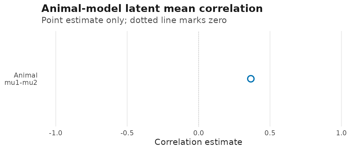

Single-row point plot for the animal-model mean-mean correlation, with a hollow estimate to the right of the dotted zero reference line.

Animal-model q=2 location-location point estimate from corpairs(); the dotted vertical line marks zero correlation. Interval calibration for this intercept-only row is not yet validated.

Use relmat() when the matrix is not naturally a pedigree, tree, or spatial coordinate surface. Here Ginv is a precision matrix for experimental breeding lines, so the fitted row is a lower-level relatedness covariance rather than an animal-model covariance.

Ginv <- animal_example$Ginv

fit_relmat_q2_known <- drmTMB(
  drm_formula(
    mu1 = body_size ~ age + sex +
      relmat(1 | p | breeding_line, Q = Ginv),
    mu2 = beak_length ~ age + sex +
      relmat(1 | p | breeding_line, Q = Ginv),
    sigma1 = ~ sex,
    sigma2 = ~ sex,
    rho12 = ~ 1
  ),
  family = c(gaussian(), gaussian()),
  data = growth
)

relmat_q2_pairs <- corpairs(
  fit_relmat_q2_known,
  level = "relmat"
)
relmat_q2_pairs
#>    level         group block from_dpar to_dpar   from_coef     to_coef
#> 1 relmat breeding_line     p       mu1     mu2 (Intercept) (Intercept)
#>   from_response to_response     class
#> 1     body_size beak_length mean-mean
#>                                                  parameter  estimate       min
#> 1 cor(mu1:(Intercept),mu2:(Intercept) | p | breeding_line) 0.4079354 0.4079354
#>         max n_values link_estimate  link_min  link_max modelled   conf.status
#> 1 0.4079354        1     0.4331324 0.4331324 0.4331324    FALSE not_requested
#>   interval_source
#> 1   not_available
relmat_q2_targets <- profile_targets(fit_relmat_q2_known)
relmat_q2_targets[
  grepl("relmat", relmat_q2_targets$parm),
  c("parm", "target_type", "profile_ready")
]
#>                                                                   parm
#> 13                             sd:mu:mu1:relmat(1 | p | breeding_line)
#> 14                             sd:mu:mu2:relmat(1 | p | breeding_line)
#> 15 cor:relmat:cor(mu1:(Intercept),mu2:(Intercept) | p | breeding_line)
#>    target_type profile_ready
#> 13      direct          TRUE
#> 14      direct          TRUE
#> 15      direct          TRUE

if (requireNamespace("ggplot2", quietly = TRUE)) {
  relmat_q2_display <- relmat_q2_pairs
  relmat_q2_display$display_label <- "relmat\nmu1-mu2"
  plot_corpairs(
    relmat_q2_display,
    colour = "level",
    label = "display_label",
    facet = NULL
  ) +
    ggplot2::scale_colour_manual(values = c("relmat" = "#6A6A6A")) +
    ggplot2::scale_fill_manual(values = c("relmat" = "#6A6A6A")) +
    structural_eye_theme() +
    ggplot2::labs(
      title = "Known-matrix latent mean correlation",
      subtitle = "Point estimate only; dotted line marks zero",
      x = "Correlation estimate"
    )
}
#> Warning: No shared levels found between `names(values)` of the manual scale and the
#> data's fill values.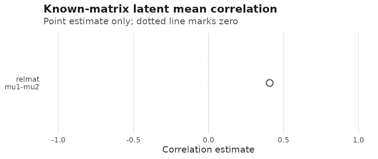

Single-row point plot for the known-matrix relmat mean-mean correlation, with a hollow estimate to the right of the dotted zero reference line.

relmat() q=2 location-location point estimate from corpairs(); the dotted vertical line marks zero correlation. Interval calibration for this intercept-only row is not yet validated.

When the relationship matrix is unavailable, fit an ordinary grouped Gaussian model as a sensitivity analysis and state the omitted structure:

fit_repeatability <- drmTMB(
  drm_formula(
    body_size ~ age + sex + (1 | individual),
    sigma ~ sex
  ),
  family = gaussian(),
  data = growth
)

check_drm(fit_repeatability)
#> <drm_check: 14 checks>
#> ok: 14; notes: 0; warnings: 0; errors: 0
#>                         check status
#>         optimizer_convergence     ok
#>              optimizer_budget     ok
#>              finite_objective     ok
#>         logsigma_clamp_active     ok
#>                fixed_gradient     ok
#>               sdreport_status     ok
#>     hessian_positive_definite     ok
#>        standard_errors_finite     ok
#>      standard_errors_inflated     ok
#>                  dropped_rows     ok
#>                positive_scale     ok
#>     random_effect_sd_boundary     ok
#>      fixed_effect_design_size     ok
#>  mu_random_effect_replication     ok
#>                                                                                   value
#>                                                                                       0
#>                                                 iterations=20; function=30; gradient=21
#>                                                                                   115.7
#>                                                                                    <NA>
#>                                                     max=0.0006233; component=beta_mu[2]
#>                                                                                      ok
#>                                                                                    TRUE
#>                                                                  range=[0.07063,0.1466]
#>                                           n_inflated=0; max_se=0.1466; median_se=0.1231
#>                                                                     nobs=160; dropped=0
#>                                                                              min=0.3998
#>                                min=0.4160; boundary=0.0001000; term=mu.(1 | individual)
#>  total_mb=0.02820; max_cols=3; largest=mu; largest_class=matrix; largest_density=0.8333
#>                                                                      (1 | individual)=4
#>                                                                                                                       message
#>                                                                                                 nlminb convergence code is 0.
#>                                           Optimizer evaluation counts recorded; no eval.max or iter.max control was supplied.
#>                                                                                      Objective and log-likelihood are finite.
#>                                                                            The log(sigma) clamp is not active at the optimum.
#>                                                 Maximum absolute fixed gradient is <= 0.001; largest component is beta_mu[2].
#>                                                                                       TMB::sdreport() completed successfully.
#>                                                                                 sdreport reports a positive-definite Hessian.
#>                                                                                  All fixed-effect standard errors are finite.
#>                                                            No fixed-effect standard error is inflated relative to the others.
#>                                                            No rows were dropped by model-frame or known-covariance filtering.
#>                                                                              All fitted scale values are finite and positive.
#>  All fitted random-effect standard deviations are finite, positive, and above the requested lower-boundary warning threshold.
#>                                                                   Dense fixed-effect design matrices are modest for this fit.
#>                                                               Every random-effect level has at least two fitted observations.

That fallback asks whether repeated observations of the same individual share a common location deviation. It does not estimate additive genetic variance, does not use pedigree relatedness among individuals, and cannot distinguish genetic resemblance from permanent environmental or measurement effects. If the scientific claim requires additive genetic variance, use the fitted animal(A/Ainv) route once the matrix is ready; report the ordinary random-effect fit only as a sensitivity check.

For matrix inputs, keep the representation explicit. A covariance matrix such as A or K is the dense VCV form. It is useful for small examples and parity checks, but it does not by itself justify large-pedigree or large-matrix claims. A precision or inverse relationship matrix such as Ainv or Q is the preferred scalable route for larger examples. The first slice validates row-name matching, determinant handling, positive definiteness, diagnostics, and recovery tests, but speed claims still need larger sparse-matrix evidence. This is the same distinction as the implemented phylogenetic tree path: users pass tree = tree, and drmTMB builds the sparse augmented A-inverse internally rather than asking users to hand-write a dense tip VCV.

Parity target for animal, spatial, and relmat

The long-term target is not just to parse animal(), spatial(), or relmat(). These routes should eventually answer the same classes of questions as the fitted phylogenetic route, whenever the corresponding dependence structure is scientifically meaningful and identifiable. The table below is a roadmap boundary, not a fitted-claim table.

Layer	Fitted phylogenetic example	Parity target for animal, spatial, and relmat
Univariate location structure	`phylo(1 \| species, tree = tree)`	`animal(1 \| individual, pedigree = pedigree)`, `spatial(1 \| site, coords = coords)`, and `relmat(1 \| line, K = K)` in `mu`
Bivariate location-location correlation	Matching labelled `phylo()` terms in `mu1` and `mu2`, reported by `corpairs()`	Matching labelled `spatial()`, `animal()`, and `relmat()` terms now fit the first q=2 slices when their coordinate or known-matrix inputs are available
Location-scale q=4 block	Matching labelled `phylo()` terms across `mu1`, `mu2`, `sigma1`, and `sigma2`	Matching labelled all-four spatial, animal, and `relmat()` blocks now fit constant q=4 location-scale covariance
Predictor-dependent structured correlation	q=2 phylogenetic `corpair(..., level = "phylogenetic") ~ ecology`	q=2 animal, spatial, and relmat `corpair()` regressions only after constant q=2 fits are stable
Direct SD surfaces	`sd_phylo()`, `sd_phylo1()`, and `sd_phylo2()`	Source-specific direct-SD siblings after naming, matrix scale, and interpretation are clear

Spatial is partway up this ladder: spatial(1 | site, coords = coords) can enter Gaussian mu, Gaussian sigma, or matching univariate mu/sigma blocks; one independent coordinate-spatial mu slope, the first bivariate coordinate-spatial q=2 mu1/mu2 covariance, and the constant q=4 location-scale covariance are fitted. Animal and relmat() now have pedigree or known-matrix Gaussian mu and sigma intercepts, matching univariate mu/sigma correlations, q1 sigma one-slope routes, matching labelled q=2 bivariate location covariance, and matching all-four constant q=4 location-scale covariance. The exact A-matrix animal and K/Q relmat sigma slopes are inference-ready with caveats; the spatial sigma-slope interval gate remains blocked. Spatial corpair(), mesh/SPDE fields, pedigree/Ainv bridge marshalling, sparse large-pedigree construction, additional multiple or labelled slope layouts outside the exact fitted ledger cells, and animal/relmat() predictor-dependent corpair() routes remain planned.

The focused animal, spatial, and relmat() pages cover the current q=2 and constant q=4 routes. A fitted animal q=4 block looks like:

fit_animal_q4 <- drmTMB(
  drm_formula(
    mu1 = body_size ~ age + sex +
      animal(1 | p | individual, pedigree = pedigree),
    mu2 = beak_length ~ age + sex +
      animal(1 | p | individual, pedigree = pedigree),
    sigma1 = ~ sex + animal(1 | p | individual, pedigree = pedigree),
    sigma2 = ~ sex + animal(1 | p | individual, pedigree = pedigree),
    rho12 = ~ 1
  ),
  family = c(gaussian(), gaussian()),
  data = growth
)

# Fitted spatial q=2 and q=4 sibling terms:
spatial(1 | p | site, coords = coords)

# Fitted relatedness q=2 and q=4 sibling terms:
relmat(1 | p | line, K = G)
relmat(1 | p | line, Q = Ginv)

The next richer animal, spatial, and relmat() targets are structured slopes and predictor-dependent structured correlations, which remain planned.

Current implementation status

This page separates the fitted paths from the roadmap. The fitted structural pieces are useful, but they are not yet the full animal, phylo, spatial, phylo+spatial, and relmat() location-scale-coscale ladder.

Model piece	Status	What it means
`animal(1 \| individual, pedigree = pedigree)`	Implemented first slice	A univariate Gaussian `mu` random intercept using a dense additive relationship matrix built from `id`, `dam`, and `sire` pedigree columns. Sparse large-pedigree precision construction remains planned.
`animal(1 \| individual, A = A)` or `animal(1 \| individual, Ainv = Ainv)`	Implemented first slice	A univariate Gaussian `mu` random intercept using a precomputed additive relatedness or inverse-relatedness matrix. Use `pedigree`, `A`, or `Ainv`; keep `V` for known sampling covariance in meta-analysis.
`animal(1 + x \| individual, pedigree = pedigree)` or `animal(1 + x \| individual, Ainv = Ainv)`	Implemented first one-slope slice	One trait has independent animal-model intercept and numeric slope fields in the location predictor. The two fields have separate SDs and do not estimate an intercept-slope correlation.
Matching labelled `animal(1 \| p \| individual, pedigree = pedigree)`, `animal(1 \| p \| individual, A = A)`, or `animal(1 \| p \| individual, Ainv = Ainv)` terms in bivariate `mu1` and `mu2`	Implemented first q=2 slice	Two Gaussian responses have correlated animal-model location deviations from the same pedigree-derived or known matrix. `corpairs(level = "animal")` reports this mean-mean row separately from residual `rho12`.
`phylo(1 \| species, tree = tree)` in univariate `mu`	Implemented	One trait has a phylogenetic random intercept in the location predictor.
`phylo(1 + x \| species, tree = tree)` in univariate `mu`	Implemented first one-slope slice	One trait has independent phylogenetic intercept and numeric slope fields in the location predictor. The two fields share the same tree-derived covariance, have separate SDs, and do not estimate an intercept-slope correlation.
Matching `phylo(1 \| species, tree = tree)` terms in bivariate `mu1` and `mu2`	Implemented first slice	Two traits have correlated phylogenetic location deviations; `corpairs(level = "phylogenetic")` reports the mean-mean row separately from residual `rho12`.
Matching labelled `phylo(1 \| p \| species, tree = tree)` terms in bivariate `mu1` and `mu2`	Implemented	The label is preserved in SD names, the fitted mean-mean correlation, `corpairs(block = "p")`, and profile-target names.
Ordinary `(1 \| p \| id)` terms in all four bivariate `mu1`, `mu2`, `sigma1`, and `sigma2` formulas	Implemented first slice	One ordinary q=4 group block estimates six latent location-location, location-scale, and scale-scale correlations.
Matching labelled `phylo()` terms in all four bivariate `mu1`, `mu2`, `sigma1`, and `sigma2` formulas	Implemented first slice	One constant q=4 phylogenetic block estimates four endpoint SDs and six latent correlations: one location-location, four location-scale, and one scale-scale. Partial, unlabelled, mismatched, and slope forms remain rejected.
`sd_phylo(species) ~ z`	Implemented for univariate Gaussian `mu`	This is the separate Box 1 direct-SD family: species-level predictors model the SD of a phylogenetic location random effect at observed tips.
`sd_phylo1(species) ~ z1` / `sd_phylo2(species) ~ z2`	Implemented for bivariate `mu1`/`mu2`	Response-specific species-level predictors model the SD surfaces of the two phylogenetic location random effects. This remains a Family B direct-SD model, not a residual `sigma1`/`sigma2` model and not a q=4 location-scale block.
`corpair(species, level = "phylogenetic", block = "p", from = "mu1", to = "mu2") ~ ecology`	Implemented for q=2 `mu1`/`mu2`	Species-level predictors model the same-species latent phylogenetic location-location correlation through a positive-definite two-field loading contract. `corpairs(level = "phylogenetic")` reports the modelled response-scale mean, range, and number of species values.
`spatial(1 \| site, coords = coords)`	Implemented first slice	One trait has a coordinate-based spatial random intercept in the location predictor. This is a fixed coordinate covariance foundation, not the future mesh/SPDE path.
`spatial(1 + x \| site, coords = coords)`	Implemented first one-slope slice	One trait has independent coordinate-spatial intercept and numeric slope fields in the location predictor. The two fields share the same coordinate precision, have separate SDs, and do not estimate an intercept-slope correlation.
Matching `spatial(1 \| p \| site, coords = coords)` terms in bivariate `mu1` and `mu2`	Implemented first q=2 slice	Two Gaussian responses have correlated coordinate-spatial location deviations. `corpairs(level = "spatial")` and `summary()$covariance` report this mean-mean row separately from residual `rho12`.
Matching labelled `spatial()` terms in all four bivariate `mu1`, `mu2`, `sigma1`, and `sigma2` formulas	Implemented first q=4 slice	Two Gaussian responses have a constant coordinate-spatial location-scale covariance block with four endpoint SDs and six derived latent spatial correlations.
`phylo(1 \| species, tree = tree) + spatial(1 \| site, coords = coords)` in the same `mu` formula	Planned	This is the intended third structural-dependence route, but the fitter currently stops with a planned-feature message because multiple structural `mu` layers need their own identifiability checks.
`relmat(1 \| id, K = K)` or `relmat(1 \| id, Q = Q)`	Implemented first slice	A lower-level Gaussian `mu` random intercept for user-supplied latent relatedness covariance or precision matrices.
`relmat(1 + x \| id, K = K)` or `relmat(1 + x \| id, Q = Q)`	Implemented first one-slope slice	One trait has independent known-matrix intercept and numeric slope fields in the location predictor. The two fields have separate SDs and do not estimate an intercept-slope correlation.
Matching labelled `relmat(1 \| p \| id, K = K)` or `relmat(1 \| p \| id, Q = Q)` terms in bivariate `mu1` and `mu2`	Implemented first q=2 slice	Two Gaussian responses have correlated lower-level known-relatedness location deviations from the same matrix. `corpairs(level = "relmat")` reports this mean-mean row separately from residual `rho12`.
`spatial(1 \| site, mesh = mesh)`	Planned	Mesh inputs will provide expert control for the scalable SPDE/GMRF spatial path.

The fitted q=2 phylogenetic correlation-regression syntax is:

corpair(species, level = "phylogenetic", block = "p",
        from = "mu1", to = "mu2") ~ ecology

The predictor-dependent q=4 extensions remain planned:

# Planned q=4 extensions:
corpair(species, level = "phylogenetic", block = "p",
        from = "mu1", to = "sigma1") ~ ecology
corpair(species, level = "phylogenetic", block = "p",
        from = "mu1", to = "sigma2") ~ ecology
corpair(species, level = "phylogenetic", block = "p",
        from = "mu2", to = "sigma1") ~ ecology
corpair(species, level = "phylogenetic", block = "p",
        from = "mu2", to = "sigma2") ~ ecology
corpair(species, level = "phylogenetic", block = "p",
        from = "sigma1", to = "sigma2") ~ ecology

Those formulae are not examples to run today. They mark the intended next layer after constant phylogenetic corpairs() rows: location-location, all four location-scale pairs, and scale-scale correlation regression. The ordinary grouped corpair() implementation cannot simply be copied here, because phylogenetic effects share one tree-coupled covariance matrix rather than independent per-species 2 by 2 blocks.

The first design contract for the location-location row uses two independent unit phylogenetic fields. For species l, the ecological predictor would define rho_l = tanh(w_l^T alpha), then c_l = sqrt((1 + rho_l) / 2) and d_l = sqrt((1 - rho_l) / 2). The two location effects would be

a1_l = tau1 (c_l z1_l + d_l z2_l)
a2_l = tau2 (c_l z1_l - d_l z2_l).

This q=2 contract is for the location-location row only: mu1-mu2. Location-scale rows such as mu1-sigma2 and scale-scale rows such as sigma1-sigma2 remain deferred until the q=4 version of this positive-definite construction is designed. This q=2 contract keeps the full covariance matrix positive definite and reduces to the current constant bivariate phylogenetic covariance when all rho_l are equal. When rho_l varies by species, the model is nonstationary: it changes the tree-coupled latent covariance surface, not just a residual correlation row.

A model ladder for two traits

The safest way to read the bivariate syntax is to build the model in layers. Each layer answers a different biological or statistical question.

1. Residual correlation only

Start here when the question is whether two measured traits remain correlated within the same observation after fixed effects:

fit_resid <- drmTMB(
  drm_formula(
    mu1 = heat_tolerance ~ climate,
    mu2 = desiccation_tolerance ~ climate,
    sigma1 = ~ habitat_variability,
    sigma2 = ~ habitat_variability,
    rho12 = ~ assay_context
  ),
  family = c(gaussian(), gaussian()),
  data = tolerance
)

rho12(fit_resid)

This model has no phylogenetic random effects. The rho12() output is the residual within-observation correlation between heat tolerance and desiccation tolerance.

2. Add phylogenetic mean-mean correlation

Add matching phylo() terms to mu1 and mu2 when the question is whether related species share deviations in the two trait means:

fit_phylo_mean <- drmTMB(
  drm_formula(
    mu1 = heat_tolerance ~ climate + phylo(1 | p | species, tree = tree),
    mu2 = desiccation_tolerance ~ climate +
      phylo(1 | p | species, tree = tree),
    sigma1 = ~ habitat_variability,
    sigma2 = ~ habitat_variability,
    rho12 = ~ assay_context
  ),
  family = c(gaussian(), gaussian()),
  data = tolerance
)

corpairs(fit_phylo_mean, level = "phylogenetic")
rho12(fit_phylo_mean)

This model estimates one latent phylogenetic mean-mean correlation and one residual rho12 surface. corpairs() and rho12() answer different questions.

The coordinate-spatial sibling uses the same bivariate location layer but replaces the tree with a coordinate-derived precision:

fit_spatial_mean <- drmTMB(
  drm_formula(
    mu1 = heat_tolerance ~ climate +
      spatial(1 | p | site, coords = coords),
    mu2 = desiccation_tolerance ~ climate +
      spatial(1 | p | site, coords = coords),
    sigma1 = ~ habitat_variability,
    sigma2 = ~ habitat_variability,
    rho12 = ~ assay_context
  ),
  family = c(gaussian(), gaussian()),
  data = tolerance
)

corpairs(fit_spatial_mean, level = "spatial")
rho12(fit_spatial_mean)

Use this model when nearby sites may share paired deviations in the two response means. Use the q=4 spatial route only when the spatial question also involves constant location-scale covariance across mu1, mu2, sigma1, and sigma2. For one-response models, sigma ~ spatial(1 | site, coords = coords) fits an intercept-only residual-scale spatial field, and sigma ~ spatial(1 + x | site, coords = coords) has point-fit/extractor evidence for the exact q1 one-slope route. Its interval gate remains blocked. Predictor-dependent spatial corpair() regression, multiple or labelled spatial sigma slopes, and bivariate spatial slope blocks remain planned. Treat the displayed spatial q2 correlation as a point estimate: interval calibration for this intercept-only row is not yet validated.

3. Let species-level predictors change phylogenetic mean SDs

Use the Box 1 direct-SD family when the question is whether species-level predictors explain the magnitude of phylogenetic mean variation:

fit_phylo_sd <- drmTMB(
  drm_formula(
    mu1 = heat_tolerance ~ climate + phylo(1 | species, tree = tree),
    mu2 = desiccation_tolerance ~ climate +
      phylo(1 | species, tree = tree),
    sigma1 = ~ habitat_variability,
    sigma2 = ~ habitat_variability,
    rho12 = ~ assay_context,
    sd_phylo1(species) ~ habitat_variability_species,
    sd_phylo2(species) ~ habitat_variability_species
  ),
  family = c(gaussian(), gaussian()),
  data = tolerance
)

coef(fit_phylo_sd, "sd_phylo1(species)")
coef(fit_phylo_sd, "sd_phylo2(species)")
corpairs(fit_phylo_sd, level = "phylogenetic")

This is not a residual scale model. sd_phylo1() and sd_phylo2() model the phylogenetic location SD surfaces for the two responses. The cross-response phylogenetic mean-mean correlation remains constant and is displayed as a point estimate; this direct-SD route does not have validated interval evidence.

4. Move to a q=4 phylogenetic location-scale block

Use the q=4 block when the question is whether phylogenetic deviations in means and residual log-SDs move together:

fit_phylo_q4 <- drmTMB(
  drm_formula(
    mu1 = heat_tolerance ~ climate + phylo(1 | p | species, tree = tree),
    mu2 = desiccation_tolerance ~ climate +
      phylo(1 | p | species, tree = tree),
    sigma1 = ~ habitat_variability +
      phylo(1 | p | species, tree = tree),
    sigma2 = ~ habitat_variability +
      phylo(1 | p | species, tree = tree),
    rho12 = ~ assay_context
  ),
  family = c(gaussian(), gaussian()),
  data = tolerance
)

corpairs(fit_phylo_q4, level = "phylogenetic")
rho12(fit_phylo_q4)

This model estimates six latent phylogenetic correlations: one location-location, four location-scale, and one scale-scale. These are constant correlations in the phylogenetic random-effect covariance block. The four location-scale rows are mu1-sigma1, mu1-sigma2, mu2-sigma1, and mu2-sigma2; the two cross-trait rows can be biologically harder to explain, but they are statistically part of the same q=4 block. They are not the residual rho12 surface.

The six q=4 correlations are point estimates. Direct or fix-and-refit profile intervals for these derived rows are not yet implemented and validated.

Read the six q=4 rows as latent phylogenetic covariance summaries:

Pair	Biological reading	Common mistake
`mu1`-`mu2`	species with positive phylogenetic deviations in trait 1 also tend to have positive or negative deviations in trait 2	treating it as residual trait coupling
`mu1`-`sigma1`	the evolutionary deviation in trait 1’s mean is associated with trait 1’s residual log-SD	reporting it as a fixed `sigma1` slope
`mu1`-`sigma2`	the evolutionary deviation in trait 1’s mean is associated with trait 2’s residual log-SD	dropping the cross-trait mean-scale row from the interpretation
`mu2`-`sigma1`	the evolutionary deviation in trait 2’s mean is associated with trait 1’s residual log-SD	dropping the cross-trait mean-scale row from the interpretation
`mu2`-`sigma2`	the evolutionary deviation in trait 2’s mean is associated with trait 2’s residual log-SD	treating it as the only mean-scale pair
`sigma1`-`sigma2`	species-level residual-scale deviations co-vary across the two traits	treating it as residual `rho12`

The cross-trait rows are not optional bookkeeping. They are part of the fitted unstructured q=4 covariance block and should remain visible in examples even when the biological story is harder to tell.

5. Predictor-dependent latent phylogenetic correlations

The q=2 location-location route is fitted:

corpair(species, level = "phylogenetic", block = "p",
        from = "mu1", to = "mu2") ~ ecology

The q=4 endpoint-specific extensions are still planned:

# Planned q=4 extensions:
corpair(species, level = "phylogenetic", block = "p",
        from = "mu1", to = "sigma1") ~ ecology
corpair(species, level = "phylogenetic", block = "p",
        from = "mu1", to = "sigma2") ~ ecology
corpair(species, level = "phylogenetic", block = "p",
        from = "mu2", to = "sigma1") ~ ecology
corpair(species, level = "phylogenetic", block = "p",
        from = "mu2", to = "sigma2") ~ ecology
corpair(species, level = "phylogenetic", block = "p",
        from = "sigma1", to = "sigma2") ~ ecology

The fitted q=2 layer makes the phylogenetic location-location random-effect correlation vary with a species-level ecological predictor, analogous in spirit to rho12 = ~ assay_context for residual correlation. The implementation is not identical to residual rho12 regression: the phylogenetic likelihood must still build one positive-definite covariance matrix for all species tied together by the tree. The selected q=2 design uses a two-field loading construction, so the modelled rho_l is the same-species phylogenetic correlation while between-species covariances remain tied to the tree and become nonstationary when rho_l varies. This first implementation target is only the location-location row; location-scale and scale-scale correlation regressions are q=4 extensions and remain deferred. The explicit level = "phylogenetic" keeps this layer separate from ordinary species effects and future spatial effects. Endpoint-specific from / to syntax avoids treating all four location-scale pairs as if they had the same biological meaning. Use corpairs() for fitted constant or modelled latent phylogenetic correlations and rho12() for fitted residual correlations. The ordinary group-level q=2 analogue is: corpair(id, level = "group", block = "p", from = "mu1", to = "mu2") ~ w models the correlation between two labelled ordinary location random intercepts.

What should get 95% intervals?

There are two different kinds of “random-effect” uncertainty.

The first kind is uncertainty in the covariance parameters: random-effect SDs and correlations. These are the quantities shown by sdpars, corpars, corpairs(), and summary(fit)$covariance. The admitted interval method is row-specific rather than a blanket preference for profile likelihood. The q1 mu anchors and the exact phylo/relmat slope-only q2 mu1:x/mu2:x SD rows use the default location-axis bias-corrected, small-sample-t Wald channel; q1 sigma uses raw uncorrected log-SD Wald-z evidence and treats profile as diagnostic-only at g = 8; the Arc 1a REML cells use direct structured-SD profiles only in their tested discrete domains. Check the capability-and-limits guide for the evidence channel attached to a particular row.

The intercept-only q2 example on this page is not one of those admitted slope-only rows. Its default Wald output is diagnostic rather than a validated reporting interval:

confint(fit_phylo_mean, parm = "variance_components")

The direct Wald route uses the fitted log-SD scale for SD targets and the guarded atanh correlation-link scale for direct correlation targets before returning intervals on the reported scale. For this intercept-only q2 row, neither a finite Wald result nor an available target promotes the row beyond diagnostic-only. A targeted profile can diagnose boundary geometry when profile_targets(fit) lists the target, but it does not replace a validated channel or promote a row whose interval evidence is diagnostic-only.

For a diagnostic look at likelihood geometry, use profile_targets() to find the target name and confint(..., method = "profile") to request a diagnostic profile. The intercept-only bivariate q2 example below is diagnostic-only under both Wald and profile channels:

profile_targets(fit_phylo_mean, ready_only = TRUE)

phylo_cor <- "cor:phylo:cor(mu1:(Intercept),mu2:(Intercept) | phylo | species)"
confint(
  fit_phylo_mean,
  parm = phylo_cor,
  method = "profile",
  profile_precision = "fast"
)

Diagnostic profile rows include conf.status = "profile". They also include profile.boundary and profile.message, so an interval that reaches a lower SD boundary or approaches a correlation boundary is marked. Do not report either interval above as validated for this intercept-only q2 fit. The admitted q2 reporting channel belongs only to the exact phylo/relmat slope-only SD rows named in the capability guide. profile_precision = "fast" is a quicker diagnostic pass that uses coarser TMB::tmbprofile() controls; use default precision only when a more detailed geometry diagnosis is needed.

The second kind is uncertainty in conditional random-effect modes, such as the species-specific fitted deviations. Those intervals are useful for caterpillar plots and diagnostics, but they are not the same as intervals for phylogenetic SDs or correlations. The current priority is covariance-parameter intervals first, then conditional-mode uncertainty once the covariance interfaces are stable.

For q=4 ordinary or phylogenetic blocks, profile_targets() lists the six correlations as derived unstructured-correlation targets. They are reported as point estimates today, but direct profile intervals for all six rows are not claimed yet. The first ordinary and phylogenetic corpair() ~ w implementations are narrower: they fit only the q=2 mu1-mu2 location-location pair for matching labelled ordinary or phylogenetic random intercepts. Those direct correlation-regression paths expose link-scale fixed-effect coefficients through coef(), summary(), vcov(), and profile_targets(), while corpairs() reports the response-scale mean, minimum, maximum, and number of group-level or species-level correlation values. The following call is a geometry diagnostic at a chosen group-level predictor value; profile availability is not validated interval evidence for this row:

confint(
  fit_ord_corpair,
  parm = 'corpair(id, level = "group", block = "p", from = "mu1", to = "mu2")',
  method = "profile",
  newdata = data.frame(w = 0)
)

The animal q=2 path uses the same fitted-versus-planned distinction. Constant corpairs(level = "animal") rows are fitted for matching labelled animal(1 | p | individual, pedigree = pedigree), A, or Ainv terms, but predictor-dependent animal corpair() regression and sparse large-pedigree precision construction remain planned.

The phylogenetic q=2 path exposes the same diagnostic profiling interface, but the parm names the phylogenetic level:

confint(
  fit_phylo_corpair,
  parm = paste0(
    'corpair(species, level = "phylogenetic", block = "p", ',
    'from = "mu1", to = "mu2")'
  ),
  method = "profile",
  newdata = data.frame(ecology = 0)
)

corpairs(conf.int = TRUE) still reports newdata_required for the modelled summary row because that row averages and ranges over group-level or species-level correlation values. Neither predictor-dependent q2 example above has coverage-backed interval validation, so do not use those diagnostic profiles as reporting intervals. q=4 rows still need a fix-and-refit or reparameterized profile before 95% intervals are claimed for all six derived correlations.

Mathematical contract

The general structured-effect bridge is:

$\eta_d = \mathbf{X}_d \boldsymbol{\beta}_d + \mathbf{Z}_d \mathbf{z}, \qquad \mathbf{z} \sim \operatorname{MVN}(\mathbf{0}, \sigma_z^2 \mathbf{K}).$

Here $d$ is the distributional parameter being modelled. For the simplest fitted examples, $d = \mu$ : the structured effect is added to the mean predictor. Current Gaussian first slices also include intercept-only structured sigma terms, q1 sigma one-slope routes for all four providers, and selected bivariate covariance blocks. The phylo, A-matrix animal, and K/Q relmat sigma slopes are inference-ready with caveats; the spatial sigma-slope interval gate, additional multiple or labelled structured-sigma layouts outside the exact fitted ledger cells, and structured rho12 remain planned. For phylogenetic models, $\mathbf{K}$ is a tree-derived phylogenetic covariance matrix $\mathbf{A}$ . For spatial models, $\mathbf{K}$ will be a distance-derived matrix or an SPDE/GMRF precision.

For the implemented univariate Gaussian phylogenetic location model:

$y_i \mid \mu_i, \sigma_i \sim \operatorname{Normal}(\mu_i, \sigma_i^2),$

$\mu_i = \mathbf{x}_{\mu i}^{\top}\boldsymbol{\beta}_{\mu} + a_{species[i]}, \qquad \log(\sigma_i) = \mathbf{x}_{\sigma i}^{\top}\boldsymbol{\beta}_{\sigma},$

$\mathbf{a} \sim \operatorname{MVN}(\mathbf{0}, \sigma_{phylo}^2\mathbf{A}).$

The phylogenetic SD $\sigma_{phylo}$ measures how strongly related species remain similar in their fitted mean after the fixed effects have been included. The residual sigma remains the within-observation residual SD. These are different scale parameters.

The matching implemented R syntax is:

drmTMB(
  drm_formula(
    y ~ x1 + phylo(1 | species, tree = tree),
    sigma ~ x1
  ),
  family = gaussian(),
  data = dat
)

Worked example: thermal tolerance across species

Suppose we measure thermal tolerance for multiple observations per species and ask whether body size predicts thermal tolerance after accounting for shared ancestry. In a real analysis, tree would usually come from a phylogenetic data workflow. For this vignette, the setup code creates a small ultrametric branch-length tree so the example stays self-contained.

set.seed(31)
tree <- balanced_ultrametric_tree(16)

species_info <- data.frame(
  species = tree$tip.label,
  body_size = scale(
    rnorm(16, mean = rep(c(-0.4, 0.4), each = 8), sd = 0.35)
  )[, 1]
)

phylo_shift <- rep(c(-0.5, 0.5), each = 8) +
  rep(c(-0.18, 0.18), each = 4, length.out = 16)

n_each <- 5
dat <- species_info[rep(seq_len(nrow(species_info)), each = n_each), ]
dat$body_size <- dat$body_size + rnorm(nrow(dat), sd = 0.08)
dat$thermal_tolerance <- 1.2 + 0.45 * dat$body_size +
  phylo_shift[match(dat$species, species_info$species)] +
  rnorm(nrow(dat), sd = 0.25)

head(dat)
#>     species body_size thermal_tolerance
#> 1      sp_1 -1.296481       -0.09668096
#> 1.1    sp_1 -1.224245        0.37697808
#> 1.2    sp_1 -1.290090        0.24284232
#> 1.3    sp_1 -1.366560       -0.06074780
#> 1.4    sp_1 -1.424426       -0.09886188
#> 2      sp_2 -1.618790       -0.07958876

The fitted model follows the equation above:

fit_phylo <- drmTMB(
  drm_formula(
    thermal_tolerance ~ body_size + phylo(1 | species, tree = tree),
    sigma ~ 1
  ),
  family = gaussian(),
  data = dat
)

summary(fit_phylo)
#> <summary.drmTMB>
#> estimator: ML
#>                     estimate  std_error
#> mu:(Intercept)     1.2055884 0.14702564
#> mu:body_size       0.4899816 0.06517078
#> sigma:(Intercept) -1.4293873 0.08571324
#> Distributional, random-effect, scale, and correlation parameters:
#>                                     component  dpar               term
#> sigma                    distributional-scale sigma         (constant)
#> sd:mu:phylo(1 | species)     random-effect-sd    mu phylo(1 | species)
#>                           estimate  std_error    scale
#> sigma                    0.2394556 0.02052451 response
#> sd:mu:phylo(1 | species) 0.2986174 0.05841679 response
#> Derived summaries:
#>                                                 quantity        level   group
#> derived:phylogenetic_signal(species) phylogenetic_signal phylogenetic species
#>                                                    term  estimate
#> derived:phylogenetic_signal(species) phylo(1 | species) 0.6086378
#>                                      random_effect_variance residual_variance
#> derived:phylogenetic_signal(species)             0.08917232        0.05733898
#> logLik: -13.41
#> convergence: 0

How to read this output:

The mu:body_size row is the fixed-effect slope for body size in the mean thermal tolerance model. The sigma:(Intercept) row is the log residual SD, so exp(coef(fit_phylo, "sigma")) gives the within-observation residual SD. The phylo(1 | species) random-effect SD is $\sigma_{phylo}$ , the phylogenetic among-species SD in the mean after body size has been included.

phylo_sd <- unname(fit_phylo$sdpars$mu["phylo(1 | species)"])
residual_sd <- exp(coef(fit_phylo, "sigma")["(Intercept)"])
c(phylogenetic_sd = phylo_sd, residual_sd = residual_sd)
#>         phylogenetic_sd residual_sd.(Intercept) 
#>               0.2986174               0.2394556

In this run, related species remain similar in thermal tolerance after accounting for body size. The fitted phylogenetic SD is larger than the within-observation residual SD, so shared ancestry explains a visible part of the remaining mean-level structure.

check_drm() reports whether the optimizer, Hessian, scale, dropped-row, and phylogenetic replication checks passed:

check_drm(fit_phylo)
#> <drm_check: 15 checks>
#> ok: 15; notes: 0; warnings: 0; errors: 0
#>                      check status
#>      optimizer_convergence     ok
#>           optimizer_budget     ok
#>           finite_objective     ok
#>      logsigma_clamp_active     ok
#>             fixed_gradient     ok
#>            sdreport_status     ok
#>  hessian_positive_definite     ok
#>     standard_errors_finite     ok
#>   standard_errors_inflated     ok
#>               dropped_rows     ok
#>             positive_scale     ok
#>  random_effect_sd_boundary     ok
#>   fixed_effect_design_size     ok
#>       phylo_mu_replication     ok
#>       phylo_mu_diagnostics     ok
#>                                                                                  value
#>                                                                                      0
#>                                                iterations=19; function=28; gradient=20
#>                                                                                  13.41
#>                                                                                   <NA>
#>                                                 max=0.0000003639; component=beta_mu[2]
#>                                                                                     ok
#>                                                                                   TRUE
#>                                                                 range=[0.06517,0.1470]
#>                                         n_inflated=0; max_se=0.1470; median_se=0.08571
#>                                                                     nobs=80; dropped=0
#>                                                                             min=0.2395
#>                             min=0.2986; boundary=0.0001000; term=mu.phylo(1 | species)
#>  total_mb=0.01305; max_cols=2; largest=mu; largest_class=matrix; largest_density=1.000
#>                                                                        min_species_n=5
#>          group=species; n_species=16; min_species_n=5; phylo_sd=0.2986; sd_ratio=1.247
#>                                                                                                                       message
#>                                                                                                 nlminb convergence code is 0.
#>                                           Optimizer evaluation counts recorded; no eval.max or iter.max control was supplied.
#>                                                                                      Objective and log-likelihood are finite.
#>                                                                            The log(sigma) clamp is not active at the optimum.
#>                                                 Maximum absolute fixed gradient is <= 0.001; largest component is beta_mu[2].
#>                                                                                       TMB::sdreport() completed successfully.
#>                                                                                 sdreport reports a positive-definite Hessian.
#>                                                                                  All fixed-effect standard errors are finite.
#>                                                            No fixed-effect standard error is inflated relative to the others.
#>                                                            No rows were dropped by model-frame or known-covariance filtering.
#>                                                                              All fitted scale values are finite and positive.
#>  All fitted random-effect standard deviations are finite, positive, and above the requested lower-boundary warning threshold.
#>                                                                   Dense fixed-effect design matrices are modest for this fit.
#>                                                                  Every observed species has at least two fitted observations.
#>              The phylogenetic random effect has replicated species and a non-negligible fitted SD relative to residual scale.

Practical checks for phylogenetic fits

The public phylo() term requires an ultrametric tree with branch lengths. Users pass the tree; drmTMB builds the sparse phylogenetic precision internally. You do not need to construct the phylogenetic covariance matrix or A-inverse yourself.

If a phylogenetic fit fails before optimization, check these points first:

the tree object has class phylo;
every observed species in data$species appears in tree$tip.label;
species names use the same spelling and underscore/space convention in the data and tree;
the tree has finite positive branch lengths and is ultrametric;
the model uses an implemented syntax: Gaussian phylo() terms in the documented univariate or matching bivariate formulas, ordinary Poisson/NB2 q1 phylogenetic mu intercept-plus-one-slope terms, recovery-grade NB2 q1 phylogenetic sigma, Student-t q1 phylogenetic nu, or cumulative-logit q1 phylogenetic mu gates recorded in the live ledger.

Additional multiple or labelled phylogenetic-slope layouts outside the exact fitted ledger cells, phylogenetic slope correlations, non-Gaussian phylogenetic effects outside those exact gates, and structured effects in rho12 remain planned. Partial, unlabelled, mismatched, and slope q=4 phylogenetic location-scale forms should error clearly rather than silently fitting a different model.

Bivariate phylogenetic correlations: model layer by layer

For two Gaussian responses, drmTMB separates the residual correlation from the phylogenetic random-effect correlation. Let $\mathbf{y}_i = (y_{1i}, y_{2i})^\top$ . A bivariate phylogenetic location model can be written as:

$\mathbf{y}_i \mid \boldsymbol{\mu}_i, \boldsymbol{\Omega}_i \sim \operatorname{MVN}(\boldsymbol{\mu}_i, \boldsymbol{\Omega}_i),$

$\begin{aligned} \mu_{1i} &= \mathbf{x}_{1i}^{\top}\boldsymbol{\beta}_1 + a_{1,s[i]},\\ \mu_{2i} &= \mathbf{x}_{2i}^{\top}\boldsymbol{\beta}_2 + a_{2,s[i]}. \end{aligned}$

$\begin{aligned} \Omega_{11,i} &= \sigma_{1i}^2,\\ \Omega_{22,i} &= \sigma_{2i}^2,\\ \Omega_{12,i} &= \Omega_{21,i} = \rho_{12,i}\sigma_{1i}\sigma_{2i}. \end{aligned}$

The residual coscale formula, rho12 = ~ assay_context, models $\rho_{12,i}$ in $\boldsymbol{\Omega}_i$ . This is an observation-level residual correlation.

The phylogenetic location effects are a separate latent layer. Let $\mathbf{a}_1$ and $\mathbf{a}_2$ collect the species-level phylogenetic location effects for responses 1 and 2. If $\mathbf{A}$ is the tree-derived species correlation matrix, then:

$\begin{aligned} \operatorname{Var}(\mathbf{a}_1) &= \tau_1^2 \mathbf{A},\\ \operatorname{Var}(\mathbf{a}_2) &= \tau_2^2 \mathbf{A},\\ \operatorname{Cov}(\mathbf{a}_1, \mathbf{a}_2) &= r_{\mu_1,\mu_2}^{\mathrm{phylo}}\tau_1\tau_2\mathbf{A}. \end{aligned}$

Here $r_{\mu_1,\mu_2}^{\mathrm{phylo}}$ is the phylogenetic mean-mean correlation. It is reported by corpairs(fit, level = "phylogenetic"), not by rho12().

The matching R syntax is:

fit_biv_phylo <- drmTMB(
  drm_formula(
    mu1 = heat_tolerance ~ climate + phylo(1 | p | species, tree = tree),
    mu2 = desiccation_tolerance ~ climate +
      phylo(1 | p | species, tree = tree),
    sigma1 = ~ habitat_variability,
    sigma2 = ~ habitat_variability,
    rho12 = ~ assay_context
  ),
  family = c(gaussian(), gaussian()),
  data = tolerance
)

corpairs(fit_biv_phylo, level = "phylogenetic")
rho12(fit_biv_phylo)

In that output, corpairs() gives the constant phylogenetic correlation point estimate among species-level mean deviations. rho12() gives the fitted residual correlation for each observation, which can vary with assay_context. The intercept-only q2 row does not have validated interval evidence; a callable profile is a diagnostic, not an inference-ready claim.

This is the key implementation boundary. drmTMB can estimate latent phylogenetic correlations when the matching phylo() terms define a shared covariance block. It can also fit the first predictor-dependent latent phylogenetic correlation formula for the q=2 location-location row. In other words, rho12 = ~ assay_context is implemented for residual correlation regression, and corpair(species, level = "phylogenetic", block = "p", from = "mu1", to = "mu2") ~ ecology is implemented for species-level predictors beside matching labelled mu1 and mu2 phylo() terms. The q=4 location-scale and scale-scale correlation regressions remain planned.

The q=4 phylogenetic location-scale block extends the same idea to four endpoints. For endpoint $d \in \{\mu_1, \mu_2, \sigma_1, \sigma_2\}$ , let $u_{d,s}$ be the phylogenetic effect for species $s$ . The covariance contract is:

$\operatorname{Cov}(u_{d,s}, u_{e,t}) = \Sigma_{de}^{\mathrm{phylo}} A_{st}, \qquad d,e \in \{\mu_1, \mu_2, \sigma_1, \sigma_2\}.$

The four linear predictors then contain one endpoint-specific phylogenetic effect:

$\mu_{1i} = \mathbf{x}_{1i}^{\top}\boldsymbol{\beta}_1 + u_{\mu_1,s[i]}, \qquad \mu_{2i} = \mathbf{x}_{2i}^{\top}\boldsymbol{\beta}_2 + u_{\mu_2,s[i]},$

$\log\sigma_{1i} = \mathbf{z}_{1i}^{\top}\boldsymbol{\gamma}_1 + u_{\sigma_1,s[i]}, \qquad \log\sigma_{2i} = \mathbf{z}_{2i}^{\top}\boldsymbol{\gamma}_2 + u_{\sigma_2,s[i]}.$

The fitted $\boldsymbol{\Sigma}^{phylo}$ is written as $\mathbf{D}\mathbf{R}\mathbf{D}$ , where $\mathbf{D}$ contains four phylogenetic SDs and $\mathbf{R}$ contains six latent correlations. Those six correlations are the corpairs(fit, level = "phylogenetic") rows: one location-location row, four location-scale rows, and one scale-scale row. The four location-scale rows are $u_{\mu_1}$ - $u_{\sigma_1}$ , $u_{\mu_1}$ - $u_{\sigma_2}$ , $u_{\mu_2}$ - $u_{\sigma_1}$ , and $u_{\mu_2}$ - $u_{\sigma_2}$ .

Worked example: two traits with phylogenetic location-scale covariance

Now suppose the scientific question is about two tolerance traits measured repeatedly for the same species. We want climate to explain each trait mean, habitat variability to explain each residual SD, and assay context to explain the residual within-observation correlation. We also want the species-level phylogenetic deviations in both means and both log-SDs to share one latent q=4 covariance block.

The simulated data below are deliberately small enough for the article to run. The hidden setup creates the tree and species-level phylogenetic effects; the fitted model uses only public drmTMB() syntax.

sim_q4 <- simulate_phylo_q4_traits()
tree <- sim_q4$tree
tol_dat <- sim_q4$data

head(tol_dat)
#>   species    climate habitat_variability assay_context heat_tolerance
#> 1    sp_1  0.8536583           1.3302474          -0.5    -1.26256225
#> 2    sp_1  1.4302245           0.7398460          -0.5    -0.25651175
#> 3    sp_1  2.2607858           0.9024009          -0.5     1.49317129
#> 4    sp_1  1.1587544          -1.0788332           0.5    -0.13889853
#> 5    sp_1  0.4185905          -0.6995513           0.5     0.24863253
#> 6    sp_1 -0.2717992           0.1264835           0.5    -0.07806504
#>   desiccation_tolerance
#> 1           -1.01377546
#> 2            0.05515596
#> 3           -0.71601270
#> 4           -0.55595513
#> 5           -0.22743664
#> 6           -0.04126080

The model uses the same labelled phylo() term in all four endpoints:

fit_phylo_q4 <- suppressWarnings(
  drmTMB(
    drm_formula(
      mu1 = heat_tolerance ~ climate + phylo(1 | p | species, tree = tree),
      mu2 = desiccation_tolerance ~ climate +
        phylo(1 | p | species, tree = tree),
      sigma1 = ~ habitat_variability +
        phylo(1 | p | species, tree = tree),
      sigma2 = ~ habitat_variability +
        phylo(1 | p | species, tree = tree),
      rho12 = ~ assay_context
    ),
    family = c(gaussian(), gaussian()),
    data = tol_dat,
    control = list(eval.max = 1000, iter.max = 1000)
  )
)

summary(fit_phylo_q4)
#> <summary.drmTMB>
#> estimator: ML
#>                               estimate std_error        std_error.status
#> mu1:(Intercept)             0.12404011        NA sdreport_non_pd_hessian
#> mu1:climate                 0.25588984        NA sdreport_non_pd_hessian
#> mu2:(Intercept)            -0.36344078        NA sdreport_non_pd_hessian
#> mu2:climate                -0.25668869        NA sdreport_non_pd_hessian
#> sigma1:(Intercept)         -1.04050450        NA sdreport_non_pd_hessian
#> sigma1:habitat_variability  0.13799113        NA sdreport_non_pd_hessian
#> sigma2:(Intercept)         -1.31598087        NA sdreport_non_pd_hessian
#> sigma2:habitat_variability -0.12081564        NA sdreport_non_pd_hessian
#> rho12:(Intercept)           0.09221661        NA sdreport_non_pd_hessian
#> rho12:assay_context        -0.15289535        NA sdreport_non_pd_hessian
#> Distributional, random-effect, scale, and correlation parameters:
#>                                                                                    component
#> sd:mu:mu1:phylo(1 | p | species)                                            random-effect-sd
#> sd:mu:mu2:phylo(1 | p | species)                                            random-effect-sd
#> sd:mu:sigma1:phylo(1 | p | species)                                         random-effect-sd
#> sd:mu:sigma2:phylo(1 | p | species)                                         random-effect-sd
#> cor:phylo:cor(mu1:(Intercept),mu2:(Intercept) | p | species)       random-effect-correlation
#> cor:phylo:cor(mu1:(Intercept),sigma1:(Intercept) | p | species)    random-effect-correlation
#> cor:phylo:cor(mu1:(Intercept),sigma2:(Intercept) | p | species)    random-effect-correlation
#> cor:phylo:cor(mu2:(Intercept),sigma1:(Intercept) | p | species)    random-effect-correlation
#> cor:phylo:cor(mu2:(Intercept),sigma2:(Intercept) | p | species)    random-effect-correlation
#> cor:phylo:cor(sigma1:(Intercept),sigma2:(Intercept) | p | species) random-effect-correlation
#> fitted:sigma1                                                           distributional-scale
#> fitted:sigma2                                                           distributional-scale
#> fitted:rho12                                                            residual-correlation
#>                                                                      dpar
#> sd:mu:mu1:phylo(1 | p | species)                                       mu
#> sd:mu:mu2:phylo(1 | p | species)                                       mu
#> sd:mu:sigma1:phylo(1 | p | species)                                    mu
#> sd:mu:sigma2:phylo(1 | p | species)                                    mu
#> cor:phylo:cor(mu1:(Intercept),mu2:(Intercept) | p | species)        phylo
#> cor:phylo:cor(mu1:(Intercept),sigma1:(Intercept) | p | species)     phylo
#> cor:phylo:cor(mu1:(Intercept),sigma2:(Intercept) | p | species)     phylo
#> cor:phylo:cor(mu2:(Intercept),sigma1:(Intercept) | p | species)     phylo
#> cor:phylo:cor(mu2:(Intercept),sigma2:(Intercept) | p | species)     phylo
#> cor:phylo:cor(sigma1:(Intercept),sigma2:(Intercept) | p | species)  phylo
#> fitted:sigma1                                                      sigma1
#> fitted:sigma2                                                      sigma2
#> fitted:rho12                                                        rho12
#>                                                                                                                        term
#> sd:mu:mu1:phylo(1 | p | species)                                                                 mu1:phylo(1 | p | species)
#> sd:mu:mu2:phylo(1 | p | species)                                                                 mu2:phylo(1 | p | species)
#> sd:mu:sigma1:phylo(1 | p | species)                                                           sigma1:phylo(1 | p | species)
#> sd:mu:sigma2:phylo(1 | p | species)                                                           sigma2:phylo(1 | p | species)
#> cor:phylo:cor(mu1:(Intercept),mu2:(Intercept) | p | species)             cor(mu1:(Intercept),mu2:(Intercept) | p | species)
#> cor:phylo:cor(mu1:(Intercept),sigma1:(Intercept) | p | species)       cor(mu1:(Intercept),sigma1:(Intercept) | p | species)
#> cor:phylo:cor(mu1:(Intercept),sigma2:(Intercept) | p | species)       cor(mu1:(Intercept),sigma2:(Intercept) | p | species)
#> cor:phylo:cor(mu2:(Intercept),sigma1:(Intercept) | p | species)       cor(mu2:(Intercept),sigma1:(Intercept) | p | species)
#> cor:phylo:cor(mu2:(Intercept),sigma2:(Intercept) | p | species)       cor(mu2:(Intercept),sigma2:(Intercept) | p | species)
#> cor:phylo:cor(sigma1:(Intercept),sigma2:(Intercept) | p | species) cor(sigma1:(Intercept),sigma2:(Intercept) | p | species)
#> fitted:sigma1                                                                                                  fitted range
#> fitted:sigma2                                                                                                  fitted range
#> fitted:rho12                                                                                                   fitted range
#>                                                                       estimate
#> sd:mu:mu1:phylo(1 | p | species)                                    0.56283742
#> sd:mu:mu2:phylo(1 | p | species)                                    0.46546831
#> sd:mu:sigma1:phylo(1 | p | species)                                 0.29622384
#> sd:mu:sigma2:phylo(1 | p | species)                                 0.17803706
#> cor:phylo:cor(mu1:(Intercept),mu2:(Intercept) | p | species)        0.57228119
#> cor:phylo:cor(mu1:(Intercept),sigma1:(Intercept) | p | species)    -0.08609142
#> cor:phylo:cor(mu1:(Intercept),sigma2:(Intercept) | p | species)    -0.31735908
#> cor:phylo:cor(mu2:(Intercept),sigma1:(Intercept) | p | species)    -0.13720281
#> cor:phylo:cor(mu2:(Intercept),sigma2:(Intercept) | p | species)     0.48759390
#> cor:phylo:cor(sigma1:(Intercept),sigma2:(Intercept) | p | species)  0.41827625
#> fitted:sigma1                                                       0.33801985
#> fitted:sigma2                                                       0.26609205
#> fitted:rho12                                                        0.09142517
#>                                                                       minimum
#> sd:mu:mu1:phylo(1 | p | species)                                           NA
#> sd:mu:mu2:phylo(1 | p | species)                                           NA
#> sd:mu:sigma1:phylo(1 | p | species)                                        NA
#> sd:mu:sigma2:phylo(1 | p | species)                                        NA
#> cor:phylo:cor(mu1:(Intercept),mu2:(Intercept) | p | species)               NA
#> cor:phylo:cor(mu1:(Intercept),sigma1:(Intercept) | p | species)            NA
#> cor:phylo:cor(mu1:(Intercept),sigma2:(Intercept) | p | species)            NA
#> cor:phylo:cor(mu2:(Intercept),sigma1:(Intercept) | p | species)            NA
#> cor:phylo:cor(mu2:(Intercept),sigma2:(Intercept) | p | species)            NA
#> cor:phylo:cor(sigma1:(Intercept),sigma2:(Intercept) | p | species)         NA
#> fitted:sigma1                                                      0.14051402
#> fitted:sigma2                                                      0.15222674
#> fitted:rho12                                                       0.01576761
#>                                                                      maximum
#> sd:mu:mu1:phylo(1 | p | species)                                          NA
#> sd:mu:mu2:phylo(1 | p | species)                                          NA
#> sd:mu:sigma1:phylo(1 | p | species)                                       NA
#> sd:mu:sigma2:phylo(1 | p | species)                                       NA
#> cor:phylo:cor(mu1:(Intercept),mu2:(Intercept) | p | species)              NA
#> cor:phylo:cor(mu1:(Intercept),sigma1:(Intercept) | p | species)           NA
#> cor:phylo:cor(mu1:(Intercept),sigma2:(Intercept) | p | species)           NA
#> cor:phylo:cor(mu2:(Intercept),sigma1:(Intercept) | p | species)           NA
#> cor:phylo:cor(mu2:(Intercept),sigma2:(Intercept) | p | species)           NA
#> cor:phylo:cor(sigma1:(Intercept),sigma2:(Intercept) | p | species)        NA
#> fitted:sigma1                                                      0.6191785
#> fitted:sigma2                                                      0.4034128
#> fitted:rho12                                                       0.1670827
#>                                                                       scale
#> sd:mu:mu1:phylo(1 | p | species)                                   response
#> sd:mu:mu2:phylo(1 | p | species)                                   response
#> sd:mu:sigma1:phylo(1 | p | species)                                response
#> sd:mu:sigma2:phylo(1 | p | species)                                response
#> cor:phylo:cor(mu1:(Intercept),mu2:(Intercept) | p | species)       response
#> cor:phylo:cor(mu1:(Intercept),sigma1:(Intercept) | p | species)    response
#> cor:phylo:cor(mu1:(Intercept),sigma2:(Intercept) | p | species)    response
#> cor:phylo:cor(mu2:(Intercept),sigma1:(Intercept) | p | species)    response
#> cor:phylo:cor(mu2:(Intercept),sigma2:(Intercept) | p | species)    response
#> cor:phylo:cor(sigma1:(Intercept),sigma2:(Intercept) | p | species) response
#> fitted:sigma1                                                      response
#> fitted:sigma2                                                      response
#> fitted:rho12                                                       response
#> Random-effect covariance summaries:
#>          level   group block from_dpar to_dpar       class correlation
#> 1 phylogenetic species     p       mu1     mu2   mean-mean  0.57228119
#> 2 phylogenetic species     p       mu1  sigma1  mean-scale -0.08609142
#> 3 phylogenetic species     p       mu1  sigma2  mean-scale -0.31735908
#> 4 phylogenetic species     p       mu2  sigma1  mean-scale -0.13720281
#> 5 phylogenetic species     p       mu2  sigma2  mean-scale  0.48759390
#> 6 phylogenetic species     p    sigma1  sigma2 scale-scale  0.41827625
#>     from_sd     to_sd  covariance
#> 1 0.5628374 0.4654683  0.14992793
#> 2 0.5628374 0.2962238 -0.01435367
#> 3 0.5628374 0.1780371 -0.03180126
#> 4 0.4654683 0.2962238 -0.01891791
#> 5 0.4654683 0.1780371  0.04040720
#> 6 0.2962238 0.1780371  0.02205940
#> logLik: -173.1
#> convergence: 1

The fixed-effect rows answer the distributional-regression questions. The mu1:climate and mu2:climate rows are mean effects. The sigma1:habitat_variability and sigma2:habitat_variability rows are effects on log residual SD. The rho12:assay_context row is the residual coscale effect: it changes the residual correlation between the two traits within the same observation.

The phylogenetic q=4 block is a different layer. Use corpairs() to read the latent species-level correlations:

corpairs(fit_phylo_q4, level = "phylogenetic")
#>          level   group block from_dpar to_dpar   from_coef     to_coef
#> 1 phylogenetic species     p       mu1     mu2 (Intercept) (Intercept)
#> 2 phylogenetic species     p       mu1  sigma1 (Intercept) (Intercept)
#> 3 phylogenetic species     p       mu1  sigma2 (Intercept) (Intercept)
#> 4 phylogenetic species     p       mu2  sigma1 (Intercept) (Intercept)
#> 5 phylogenetic species     p       mu2  sigma2 (Intercept) (Intercept)
#> 6 phylogenetic species     p    sigma1  sigma2 (Intercept) (Intercept)
#>           from_response           to_response       class
#> 1        heat_tolerance desiccation_tolerance   mean-mean
#> 2        heat_tolerance        heat_tolerance  mean-scale
#> 3        heat_tolerance desiccation_tolerance  mean-scale
#> 4 desiccation_tolerance        heat_tolerance  mean-scale
#> 5 desiccation_tolerance desiccation_tolerance  mean-scale
#> 6        heat_tolerance desiccation_tolerance scale-scale
#>                                                  parameter    estimate
#> 1       cor(mu1:(Intercept),mu2:(Intercept) | p | species)  0.57228119
#> 2    cor(mu1:(Intercept),sigma1:(Intercept) | p | species) -0.08609142
#> 3    cor(mu1:(Intercept),sigma2:(Intercept) | p | species) -0.31735908
#> 4    cor(mu2:(Intercept),sigma1:(Intercept) | p | species) -0.13720281
#> 5    cor(mu2:(Intercept),sigma2:(Intercept) | p | species)  0.48759390
#> 6 cor(sigma1:(Intercept),sigma2:(Intercept) | p | species)  0.41827625
#>           min         max n_values link_estimate    link_min    link_max
#> 1  0.57228119  0.57228119        1    0.65090926  0.65090926  0.65090926
#> 2 -0.08609142 -0.08609142        1   -0.08630515 -0.08630515 -0.08630515
#> 3 -0.31735908 -0.31735908        1   -0.32870802 -0.32870802 -0.32870802
#> 4 -0.13720281 -0.13720281        1   -0.13807373 -0.13807373 -0.13807373
#> 5  0.48759390  0.48759390        1    0.53289954  0.53289954  0.53289954
#> 6  0.41827625  0.41827625        1    0.44560142  0.44560142  0.44560142
#>   modelled   conf.status interval_source
#> 1    FALSE not_requested   not_available
#> 2    FALSE not_requested   not_available
#> 3    FALSE not_requested   not_available
#> 4    FALSE not_requested   not_available
#> 5    FALSE not_requested   not_available
#> 6    FALSE not_requested   not_available

Those six rows are not residual correlations. The mean-mean row asks whether species that are phylogenetically high for heat tolerance also tend to be high for desiccation tolerance. The four mean-scale rows ask whether evolutionary deviations in means are associated with evolutionary deviations in variability: same-trait pairs (mu1-sigma1, mu2-sigma2) and cross-trait pairs (mu1-sigma2, mu2-sigma1). The cross-trait rows are statistically valid q=4 covariance rows, but their biological interpretation should be written with extra care.

The scale-scale row asks whether the two traits’ phylogenetic log-SD deviations move together. These q=4 rows are point estimates and remain derived targets until a direct or fix-and-refit profile is implemented and validated.

For a compact scalar view of the residual layer, use rho12():

range(rho12(fit_phylo_q4))
#> [1] 0.01576761 0.16708274

check_drm() keeps these layers separate. In small examples, q=4 models can warn about optimizer convergence even when gradients, Hessian status, and q=4 covariance diagnostics are acceptable. Treat this article fit as an output map; for scientific inference, inspect the full diagnostic table and use larger datasets or simpler covariance structure when needed.

q4_check <- check_drm(fit_phylo_q4)
q4_check[q4_check$check %in% c(
  "optimizer_convergence",
  "fixed_gradient",
  "hessian_positive_definite",
  "biv_phylo_q4_covariance"
), ]
#> <drm_check: 4 checks>
#> ok: 2; notes: 0; warnings: 2; errors: 0
#>                      check  status
#>      optimizer_convergence warning
#>             fixed_gradient      ok
#>  hessian_positive_definite warning
#>    biv_phylo_q4_covariance      ok
#>                                                                                                                                                                                value
#>                                                                                                                                                                                    1
#>                                                                                                                                                max=0.00007279; component=beta_mu2[2]
#>                                                                                                                                                                                FALSE
#>  group=species; block=p; covariance_mode=unstructured; q=4; n_species=32; min_species_n=6; min_location_sd_ratio=1.665; min_log_sigma_sd=0.1780; max_abs_cor=0.5723; boundary=0.9800
#>                                                                                                                                                message
#>                                                                                                   nlminb convergence message: singular convergence (7)
#>                                                                         Maximum absolute fixed gradient is <= 0.001; largest component is beta_mu2[2].
#>                                                                                                  sdreport does not report a positive-definite Hessian.
#>  Phylogenetic q4 location-scale covariance has replicated levels, non-negligible fitted component SDs, and latent correlations away from the boundary.

The fitted q=4 correlations are point summaries. They are listed in profile_targets() as derived theta_phylo targets, not as direct profile-ready intervals:

subset(
  profile_targets(fit_phylo_q4),
  startsWith(parm, "cor:phylo:"),
  select = c(parm, target_type, profile_ready, profile_note)
)
#>                                                                  parm
#> 15       cor:phylo:cor(mu1:(Intercept),mu2:(Intercept) | p | species)
#> 16    cor:phylo:cor(mu1:(Intercept),sigma1:(Intercept) | p | species)
#> 17    cor:phylo:cor(mu1:(Intercept),sigma2:(Intercept) | p | species)
#> 18    cor:phylo:cor(mu2:(Intercept),sigma1:(Intercept) | p | species)
#> 19    cor:phylo:cor(mu2:(Intercept),sigma2:(Intercept) | p | species)
#> 20 cor:phylo:cor(sigma1:(Intercept),sigma2:(Intercept) | p | species)
#>    target_type profile_ready                     profile_note
#> 15     derived         FALSE derived_unstructured_correlation
#> 16     derived         FALSE derived_unstructured_correlation
#> 17     derived         FALSE derived_unstructured_correlation
#> 18     derived         FALSE derived_unstructured_correlation
#> 19     derived         FALSE derived_unstructured_correlation
#> 20     derived         FALSE derived_unstructured_correlation

The q=2 predictor-dependent latent phylogenetic correlation is fitted for the location-location row. The extractor is corpairs(), and the formula syntax is singular:

corpair(species, level = "phylogenetic", block = "p",
        from = "mu1", to = "mu2") ~ w

The predictor-dependent q=4 extensions remain planned:

# Planned q=4 extensions:
corpair(species, level = "phylogenetic", block = "p",
        from = "mu1", to = "sigma1") ~ w
corpair(species, level = "phylogenetic", block = "p",
        from = "mu1", to = "sigma2") ~ w
corpair(species, level = "phylogenetic", block = "p",
        from = "mu2", to = "sigma1") ~ w
corpair(species, level = "phylogenetic", block = "p",
        from = "mu2", to = "sigma2") ~ w
corpair(species, level = "phylogenetic", block = "p",
        from = "sigma1", to = "sigma2") ~ w

This endpoint naming matters because the cross-trait mean-scale pairs can be biologically harder to interpret than same-trait pairs. Use rho12 = ~ assay_context for residual correlation predictors. Use corpairs(fit, level = "phylogenetic") to extract fitted constant or modelled latent phylogenetic correlations.

Implemented third route: coordinate spatial intercepts and one slope

Spatial fields are the third route in the structural-dependence ladder. They are deliberately shaped to look parallel to phylogenetic effects, but they use site coordinates rather than a tree. The first fitted paths are coordinate-based univariate Gaussian mu coefficient fields: a random intercept, and one independent random slope for a numeric predictor. The example below keeps the data deliberately small so the models can be rebuilt inside the article:

spatial_example <- simulate_spatial_location_data()
spatial_dat <- spatial_example$data
coords <- spatial_example$coords

fit_spatial <- drmTMB(
  drm_formula(
    y ~ depth + temp + spatial(1 | site, coords = coords),
    sigma ~ depth
  ),
  family = gaussian(),
  data = spatial_dat
)

The fitted spatial SD is a structured location-scale component, not the residual sigma. The conditional spatial effects are site-level deviations in the location predictor, after the fixed effects and residual scale have been estimated:

fit_spatial$sdpars$mu
#> spatial(1 | site) 
#>         0.3808036
head(ranef(fit_spatial, "spatial_mu")$terms[[1]])
#>     site_1     site_2     site_3     site_4     site_5     site_6 
#> -0.2640539 -0.4642452 -0.0359260 -0.1560390 -0.3023818  0.2240647
profile_targets(fit_spatial, ready_only = TRUE)[
  grep("spatial", profile_targets(fit_spatial, ready_only = TRUE)$parm),
  c("parm", "estimate", "profile_ready")
]
#>                      parm  estimate profile_ready
#> 6 sd:mu:spatial(1 | site) 0.3808036          TRUE

When the biological question is whether a local environmental gradient has a different slope in different parts of the sampled landscape, add one numeric coefficient inside the spatial() term:

fit_spatial_slope <- drmTMB(
  drm_formula(
    y ~ depth + temp + spatial(1 + depth | site, coords = coords),
    sigma ~ depth
  ),
  family = gaussian(),
  data = spatial_dat
)

fit_spatial_slope$sdpars$mu
#>         spatial(1 | site) spatial(0 + depth | site) 
#>              3.808036e-01              4.396188e-06
names(ranef(fit_spatial_slope, "spatial_mu")$terms)
#> [1] "spatial(1 | site)"         "spatial(0 + depth | site)"

The two SDs answer different biological questions. spatial(1 | site) is the amount of smooth site-to-site variation in the expected response after the fixed effects. spatial(0 + depth | site) is the amount of smooth site-to-site variation in the depth effect. Large slope SD means the fitted depth-response gradient changes across the coordinate surface; it is not a residual correlation and it is not the residual scale sigma.

Before interpreting the spatial SD or mapped site effects, inspect the spatial diagnostic row. It is deliberately named spatial_mu_diagnostics, not phylo_mu_replication, because the fitted layer is a coordinate site field:

spatial_check <- check_drm(fit_spatial)
spatial_check[spatial_check$check %in% c(
  "optimizer_convergence",
  "fixed_gradient",
  "hessian_positive_definite",
  "spatial_mu_diagnostics"
), ]
#> <drm_check: 4 checks>
#> ok: 4; notes: 0; warnings: 0; errors: 0
#>                      check status
#>      optimizer_convergence     ok
#>             fixed_gradient     ok
#>  hessian_positive_definite     ok
#>     spatial_mu_diagnostics     ok
#>                                                                                       value
#>                                                                                           0
#>                                                    max=0.000008559; component=beta_sigma[1]
#>                                                                                        TRUE
#>  group=site; n_sites=12; min_site_n=6; coord_range=1.475; spatial_sd=0.3808; sd_ratio=1.214
#>                                                                                                                      message
#>                                                                                                nlminb convergence code is 0.
#>                                             Maximum absolute fixed gradient is <= 0.001; largest component is beta_sigma[1].
#>                                                                                sdreport reports a positive-definite Hessian.
#>  The coordinate spatial random intercept has replicated sites and a non-negligible fitted SD relative to the residual scale.

The spatial row reports the number of fitted sites, the minimum number of observations per site, the coordinate range used by the fixed exponential covariance, the fitted spatial SD, and the ratio between the spatial SD and the residual scale. A note is not a failed model. It tells you to be cautious when a site is singly observed or when the spatial field is tiny relative to unstructured residual variation.

The fitted coords path accepts either one row per site or one row per observation, provided coordinates are constant within each site. Internally, the coordinate path builds a fixed exponential covariance from pairwise site distances, inverts it to a precision matrix, and estimates one spatial SD for each fitted spatial coefficient. The intercept model estimates one field. The one-slope model spatial(1 + depth | site, coords = coords) estimates two independent fields: spatial(1 | site) for site intercept deviations and spatial(0 + depth | site) for site-specific depth slopes. These two fields share the same coordinate precision but have separate SDs and no intercept-slope corpair() row. This is a small-data foundation and recovery target, not the scalable mesh/SPDE implementation. The conditional spatial effects from ranef() are shrunken site deviations in the location predictor after the fixed effects and the spatial covariance have been estimated.

The planned mesh argument plays a different role. A mesh is the computational scaffold for an SPDE/GMRF field: a triangular network of vertices where the latent spatial field is represented and then projected back to observations. Users should not interpret mesh vertices as biological sampling units; they are numerical support points for the spatial surface. In other words, a mesh is not required by the idea of spatial dependence itself. It is required by the scalable SPDE/GMRF approximation. The friendly API should let users start with coords = coords; mesh = mesh is the expert route for reproducible control over boundaries, barriers, coastlines, or uneven sampling.

The spatial term is deliberately parallel to the phylogenetic term:

# implemented for Gaussian mu/sigma intercepts and matching bivariate blocks
phylo(1 | species, tree = tree)
# implemented for one numeric Gaussian mu slope
phylo(1 + x | species, tree = tree)
# implemented for Gaussian mu/sigma intercepts and matching bivariate blocks
spatial(1 | site, coords = coords)
# implemented for one numeric Gaussian mu slope
spatial(1 + x | site, coords = coords)
# planned
spatial(1 | site, mesh = mesh)

The mathematical role is the same: add structured Gaussian coefficient fields to a distributional predictor. The computational route differs. phylo() starts from an ultrametric tree with branch lengths and builds a sparse tree-derived precision. The first spatial() slice starts from coordinates and builds a fixed coordinate precision; the future mesh path will build an SPDE/GMRF precision.

The computational plan is to keep using sparse A-inverse ideas for phylogeny and add SPDE/GMRF structure for spatial fields. The spatial route should cite the SPDE/GMRF method literature and the software it builds on. The key methodological reference is Lindgren, Rue, and Lindstrom (2011), who connected Gaussian fields to sparse GMRFs through the SPDE approach (doi:10.1111/j.1467-9868.2011.00777.x). The ecological TMB precedent is sdmTMB, described in its Journal of Statistical Software paper as a package for spatial and spatiotemporal GLMMs using TMB, fmesher, latent GMRFs, and the SPDE approach. If drmTMB imports fmesher or asks users to pass fmesher mesh objects, the website and paper should also tell users to cite fmesher as software. Any code selectively ported from gllvmTMB, sdmTMB, fmesher, or INLA-related sources must be recorded in inst/COPYRIGHTS before the spatial feature is called complete.

Structured random slopes are staged more conservatively than ordinary grouped random slopes. Coordinate spatial and phylogenetic Gaussian mu have first one-slope paths, and q1 structured sigma one-slope paths fit for phylo/spatial/animal/relmat. The phylo, A-matrix animal, and K/Q relmat sigma slopes are inference-ready with caveats; spatial is point-fit/extractor only. These paths are deliberately independent: each returns separate SDs and no intercept-slope corpair() row. Additional multiple or labelled structured-slope layouts outside the exact fitted ledger cells, mesh/SPDE slopes, and structured slope correlations remain later gates. The combined phylogeny-plus-spatial route should be a separate additive-block model with a phylogenetic field and a spatial field, not one large cross-factor covariance model. A more interesting future two-response target is the slope1-slope2 correlation for the same covariate across traits, the plasticity-syndrome question described by O’Dea, Noble, and Nakagawa (2021).

Meta-analysis and future bivariate structure

In meta-analysis, the separation among known sampling covariance, phylogenetic dependence, and spatial dependence is especially transparent:

$\begin{aligned} e &\sim \operatorname{MVN}(\mathbf{0}, V) &&\text{known sampling covariance},\\ p_{species} &\sim \operatorname{MVN}(\mathbf{0}, \sigma_{phylo}^2 A) &&\text{phylogenetic structure},\\ \ell_{location} &\sim \operatorname{MVN}(\mathbf{0}, \sigma_{space}^2 M) &&\text{spatial structure}. \end{aligned}$

The known matrix V handles sampling uncertainty. The phylogenetic and spatial terms add extra biological or environmental dependence after that known uncertainty has been included. The same design will let drmTMB support structured Gaussian meta-analysis while keeping ecological and evolutionary meta-analyses readable.

The first phylogenetic target is the location-scale model. In bivariate Gaussian models, matching mu1/mu2 phylogenetic location terms estimate the mean-mean phylogenetic correlation. Matching labelled phylo() terms across mu1, mu2, sigma1, and sigma2 now fit the first constant q=4 phylogenetic location-scale block: one location-location row, four location-scale rows, and one scale-scale row in corpairs(level = "phylogenetic"). The six q=4 correlations are latent phylogenetic random-effect correlations, not residual rho12.

The first fitted bivariate phylogenetic location-coscale syntax looks like this:

fit_biv_phylo <- drmTMB(
  formula = drm_formula(
    mu1 = log_body_mass ~ lifestyle + phylo(1 | species, tree = tree),
    mu2 = log_litter_size ~ lifestyle + phylo(1 | species, tree = tree),
    sigma1 = ~ lifestyle,
    sigma2 = ~ lifestyle,
    rho12 = ~ lifestyle
  ),
  family = c(gaussian(), gaussian()),
  data = mammals
)

This syntax fits correlated phylogenetic random intercepts in mu1 and mu2. It estimates two phylogenetic location SDs and one phylogenetic mean-mean correlation. The sigma1, sigma2, and residual rho12 formulas remain ordinary fixed-effect distributional parameters in this first slice. Use phylo(1 | p | species, tree = tree) in both location formulas when you want the fitted phylogenetic mean-mean row to use a block label such as p.

The Box 1 direct-SD alternative for two responses keeps the phylogenetic effects in the location formulas, but lets species-level predictors explain the magnitude of each response’s phylogenetic location variation:

fit_biv_sd_phylo <- drmTMB(
  formula = drm_formula(
    mu1 = heat_tolerance ~ climate +
      phylo(1 | species, tree = tree),
    mu2 = desiccation_tolerance ~ climate +
      phylo(1 | species, tree = tree),
    sigma1 = ~ habitat_variability,
    sigma2 = ~ habitat_variability,
    rho12 = ~ assay_context,
    sd_phylo1(species) ~ habitat_variability_species,
    sd_phylo2(species) ~ habitat_variability_species
  ),
  family = c(gaussian(), gaussian()),
  data = tolerance
)

Here sd_phylo1(species) targets the mu1 phylogenetic location SD surface and sd_phylo2(species) targets the mu2 surface. The right-hand-side predictors must be constant within species after model-row filtering. The latent phylogenetic mean-mean correlation remains a constant fitted correlation, and rho12 remains the within-observation residual correlation:

corpairs(fit_biv_sd_phylo, level = "phylogenetic")
rho12(fit_biv_sd_phylo)

The corpairs() row is the fitted phylogenetic correlation point estimate between the two location random effects; this direct-SD route does not have validated interval evidence. The rho12() values are residual correlations between the two responses after the fitted fixed effects and phylogenetic effects have been included. Run check_drm(fit_biv_sd_phylo) before interpreting the direct-SD slopes; the diagnostic reports species replication, each fitted species-SD range, and whether any fitted direct-SD surface is non-positive or non-finite.

Mathematically, the direct-SD model replaces constant phylogenetic location SDs with species-level SD surfaces. For response $k \in \{1,2\}$ :

$\operatorname{Var}(\mathbf{a}_k) = \mathbf{D}_k(\mathbf{z})\,\mathbf{A}\,\mathbf{D}_k(\mathbf{z}), \qquad \log D_{k,ss}(\mathbf{z}) = \mathbf{z}_s^{\top}\boldsymbol{\alpha}_k.$

The current bivariate direct-SD path keeps the cross-response phylogenetic location correlation constant:

$\operatorname{Cov}(\mathbf{a}_1, \mathbf{a}_2) = r_{\mu_1,\mu_2}^{phylo} \mathbf{D}_1(\mathbf{z})\,\mathbf{A}\,\mathbf{D}_2(\mathbf{z}).$

This is why sd_phylo1(species) ~ habitat_variability_species and sd_phylo2(species) ~ habitat_variability_species answer a different question from the q=4 location-scale block. They ask whether species-level predictors change the magnitude of phylogenetic mean variation for each response. They do not put random effects into sigma1 or sigma2.

The full constant q=4 location-scale form uses an explicit covariance-block label:

fit_biv_phylo_q4 <- drmTMB(
  formula = drm_formula(
    mu1 = heat_tolerance ~ climate + phylo(1 | p | species, tree = tree),
    mu2 = desiccation_tolerance ~ climate +
      phylo(1 | p | species, tree = tree),
    sigma1 = ~ habitat_variability +
      phylo(1 | p | species, tree = tree),
    sigma2 = ~ habitat_variability +
      phylo(1 | p | species, tree = tree),
    rho12 = ~ assay_context
  ),
  family = c(gaussian(), gaussian()),
  data = tolerance
)

corpairs(fit_biv_phylo_q4, level = "phylogenetic")
rho12(fit_biv_phylo_q4)

Partial q=4 syntax, unlabelled all-four syntax, random slopes, and multiple phylogenetic blocks remain outside this first fitted path. The q=4 corpairs() output has six phylogenetic rows: one location-location row, four location-scale rows, and one scale-scale row. The four location-scale rows include both same-trait and cross-trait mean-scale pairs. These rows are the latent phylogenetic correlations among species-level effects. They are not the residual rho12 curve, which is why the example shows corpairs() and rho12() separately.

For the simpler fitted mean-mean phylogenetic correlation point estimate, use corpars$phylo, corpairs(fit_biv_phylo, level = "phylogenetic"), or summary(fit_biv_phylo)$covariance. Run check_drm(fit_biv_phylo) before interpreting that row: the current diagnostic flags phylogenetic correlations near the boundary and phylogenetic location SDs that are tiny relative to the matching residual scales. profile_targets() can expose a callable diagnostic profile target, but that does not validate an interval or promote this intercept-only q2 row. The q=4 correlations are derived from theta_phylo, so direct profile intervals for those six rows are not yet claimed:

phylo_target <- "cor:phylo:cor(mu1:(Intercept),mu2:(Intercept) | phylo | species)"

corpairs(fit_biv_phylo, level = "phylogenetic")
summary(fit_biv_phylo)$covariance
profile_targets(fit_biv_phylo)

Do not read a phylogenetic species effect as a residual observation-level correlation. The phylo() layer is species-level structure induced by the tree; residual rho12 is within-observation coupling between the two measured responses. A separate non-phylogenetic species-level block can be useful in a specialized model, but it is an advanced comparison because it tries to separate two species-level covariance layers that use the same grouping factor. That comparison should live in a dedicated identifiability example, not in this introductory ladder.

The residual rho12 term remains distinct from the phylogenetic or spatial correlation matrices. rho12 is the residual coupling between two responses at the observation level; A and M describe dependence among species or places. In future bivariate structural models, drmTMB should also estimate level-specific correlations such as phylogenetic mean-mean correlations, non-phylogenetic species correlations, spatial field correlations, and mean-scale correlations. These are not residual rho12; they should be reported as structural or group-level covariance summaries. For the univariate structural-dependence ladder, keep the implementation status visible: use animal(pedigree/A/Ainv = ...) for the animal-model first slice, use phylo() when the species tree is the fitted dependence structure, use spatial() when the site field is the fitted dependence structure, plan combined phylo() plus spatial() only after joint identifiability checks, and use relmat(K/Q = ...) for lower-level known-matrix latent random effects.