Robust continuous responses

Continuous biological and environmental measurements, such as seedling height growth in centimetres, often contain a few large residuals. They may be real rare events, short-term stress responses, field measurement problems, or individuals that experienced unmeasured conditions. A Gaussian location-scale model can still be useful, but a Student-t model asks a slightly different question: are the location and scale patterns stable when the likelihood allows heavier tails?

This article introduces the first implemented robust continuous family in drmTMB: fixed-effect Student-t location-scale-shape regression. It builds on the location-scale reading pattern from When variance carries signal and adds a third parameter. Here location means the expected response parameter mu, scale means the positive Student-t core scale sigma, and shape means the tail parameter nu. This one-response model has no coscale term; in drmTMB, coscale means modelling residual correlation, such as bivariate rho12.

Model equation and R syntax

The Student-t model has three distributional parameters:

$$\begin{aligned} \text{growth}_i \mid \mu_i, \sigma_i, \nu_i &\sim \operatorname{Student\text{-}t}(\mu_i, \sigma_i, \nu_i),\\ \mu_i &= \beta_0 + \beta_1 \text{dry}_i,\\ \log(\sigma_i) &= \gamma_0 + \gamma_1 \text{dry}_i,\\ \nu_i &= 2 + \exp(\delta_0). \end{aligned}$$

The matching drmTMB syntax is:

drmTMB(
  bf(growth ~ drought, sigma ~ drought, nu ~ 1),
  family = student(),
  data = seedlings
)

Here mu is the expected response, sigma is the Student-t scale parameter, and nu is the tail-shape parameter. When nu > 2, the residual standard deviation is sigma * sqrt(nu / (nu - 2)), so sigma should not be read as the exact residual SD unless nu is large. Smaller nu means heavier tails. Large nu means the Student-t likelihood is close to Gaussian. In drmTMB,

$$\nu_i = 2 + \exp(\eta_{\nu i}).$$

so fitted nu values stay above 2. This keeps the fitted Student-t distribution in the finite-variance region.

A seedling growth example

Suppose seedlings are grown under ambient and dry conditions, and growth is measured as height increase in centimetres. We expect drought to reduce average growth, and we also allow drought to change scale among seedlings.

library(drmTMB)
#> 
#> Attaching package: 'drmTMB'
#> The following object is masked from 'package:base':
#> 
#>     beta

set.seed(101)
n <- 180
seedlings <- data.frame(
  drought = factor(rep(c("ambient", "dry"), each = n / 2))
)
dry <- as.numeric(seedlings$drought == "dry")
mu <- 1.2 - 0.45 * dry
sigma <- exp(-1 + 0.35 * dry)
seedlings$growth <- mu + sigma * rt(n, df = 5)

In the equation above, dry_i is the model-matrix indicator for the dry treatment level. It corresponds to the droughtdry coefficient printed by R.

A Gaussian location-scale model is a useful baseline:

fit_gaussian <- drmTMB(
  bf(growth ~ drought, sigma ~ drought),
  family = gaussian(),
  data = seedlings
)

The robust version keeps the same location and scale formulas, then adds a formula for nu:

fit_student <- drmTMB(
  bf(growth ~ drought, sigma ~ drought, nu ~ 1),
  family = student(),
  data = seedlings
)

The extra line nu ~ 1 says that the tail-shape parameter is estimated as a constant across observations. Predictor-varying fixed-effect nu formulas are also supported. For example, nu ~ drought asks whether the residual tails are heavier in the dry treatment than in the ambient treatment after mu and sigma have been modelled. This first tutorial keeps nu constant so the comparison focuses on location, scale, and residual-tail assumptions.

Check the fitted robust model

Run check_drm() before interpreting the Student-t coefficients:

student_checks <- check_drm(fit_student)
student_checks
#> <drm_check: 13 checks>
#> ok: 13; notes: 0; warnings: 0; errors: 0
#>                      check status
#>      optimizer_convergence     ok
#>           optimizer_budget     ok
#>           finite_objective     ok
#>      logsigma_clamp_active     ok
#>             fixed_gradient     ok
#>            sdreport_status     ok
#>  hessian_positive_definite     ok
#>     standard_errors_finite     ok
#>   standard_errors_inflated     ok
#>               dropped_rows     ok
#>             positive_scale     ok
#>                 student_nu     ok
#>   fixed_effect_design_size     ok
#>                                                                                   value
#>                                                                                       0
#>                                                 iterations=23; function=36; gradient=24
#>                                                                                   144.6
#>                                                                                    <NA>
#>                                                   max=0.000009575; component=beta_mu[1]
#>                                                                                      ok
#>                                                                                    TRUE
#>                                                                  range=[0.04836,0.9790]
#>                                           n_inflated=0; max_se=0.9790; median_se=0.1110
#>                                                                     nobs=180; dropped=0
#>                                                                              min=0.4116
#>                                                                     range=[9.615,9.615]
#>  total_mb=0.04302; max_cols=2; largest=mu; largest_class=matrix; largest_density=0.7500
#>                                                                              message
#>                                                        nlminb convergence code is 0.
#>  Optimizer evaluation counts recorded; no eval.max or iter.max control was supplied.
#>                                             Objective and log-likelihood are finite.
#>                                   The log(sigma) clamp is not active at the optimum.
#>        Maximum absolute fixed gradient is <= 0.001; largest component is beta_mu[1].
#>                                              TMB::sdreport() completed successfully.
#>                                        sdreport reports a positive-definite Hessian.
#>                                         All fixed-effect standard errors are finite.
#>                   No fixed-effect standard error is inflated relative to the others.
#>                   No rows were dropped by model-frame or known-covariance filtering.
#>                                     All fitted scale values are finite and positive.
#>               All fitted Student-t nu values are finite and above the boundary at 2.
#>                          Dense fixed-effect design matrices are modest for this fit.
student_checks[
  student_checks$check == "student_nu",
  c("status", "value", "message")
]
#> <drm_check: 1 checks>
#> ok: 1; notes: 0; warnings: 0; errors: 0
#>  status               value
#>      ok range=[9.615,9.615]
#>                                                                 message
#>  All fitted Student-t nu values are finite and above the boundary at 2.

The student_nu row inspects fitted response-scale nu values. A near-boundary warning means the tail-shape parameter is close to 2, where the finite-variance constraint matters. A large-nu note means the Student-t fit may be close to a Gaussian fit. If nu is large, report that the Student-t fit is close to Gaussian and check whether the Gaussian and Student-t mu and sigma conclusions differ. If nu is near the boundary, inspect influential observations, compare Gaussian and Student-t conclusions, and report that the fitted tail-shape parameter is near the lower bound.

Keep the student_nu status beside AIC, coefficient, and simulation-summary tables. An ok row supports reading the fitted nu as an ordinary finite-variance Student-t shape estimate. A note or warning should travel with the result, because it changes how a reader should interpret the tail assumption even when the optimizer converged.

Interpret coefficients by parameter

Location and scale coefficients use the same formula grammar as Gaussian location-scale models:

coef(fit_student, "mu")
#> (Intercept)  droughtdry 
#>   1.2084533  -0.4493227
coef(fit_student, "sigma")
#> (Intercept)  droughtdry 
#>  -0.8877248   0.3309563
coef(fit_student, "nu")
#> (Intercept) 
#>    2.030157

The mu coefficient for droughtdry estimates the drought difference in expected growth. The sigma coefficient for droughtdry is on the log Student-t scale-parameter scale: a positive value means the fitted scale is larger under drought. The nu coefficient is on the link scale for nu = 2 + exp(eta_nu). Use prediction to read nu on the response scale:

head(predict(fit_student, dpar = "nu"))
#> [1] 9.61528 9.61528 9.61528 9.61528 9.61528 9.61528

Compare with the Gaussian model

For this simulated example, the two models share mu and sigma formulas: does drought reduce growth, and does it change scale? They differ in the residual-tail assumption.

AIC(fit_gaussian, fit_student)
#>   df      AIC
#> 1  4 299.2362
#> 2  5 299.1516

AIC is only one summary. The more important habit is to inspect whether the scientific conclusions about mu and sigma are sensitive to the residual tail assumption.

coef(fit_gaussian, "mu")
#> (Intercept)  droughtdry 
#>   1.2242784  -0.4899042
coef(fit_student, "mu")
#> (Intercept)  droughtdry 
#>   1.2084533  -0.4493227

coef(fit_gaussian, "sigma")
#> (Intercept)  droughtdry 
#>  -0.7835902   0.3472780
coef(fit_student, "sigma")
#> (Intercept)  droughtdry 
#>  -0.8877248   0.3309563

library(ggplot2)

student_plot_grid <- data.frame(
  drought = factor(c("ambient", "dry"), levels = levels(seedlings$drought))
)
student_plot_means <- rbind(
  data.frame(
    student_plot_grid,
    model = "Gaussian",
    fitted_mu = predict(fit_gaussian, newdata = student_plot_grid, dpar = "mu")
  ),
  data.frame(
    student_plot_grid,
    model = "Student-t",
    fitted_mu = predict(fit_student, newdata = student_plot_grid, dpar = "mu")
  )
)

ggplot(seedlings, aes(drought, growth, colour = drought)) +
  geom_jitter(width = 0.12, height = 0, alpha = 0.22, size = 1.1) +
  geom_point(
    data = student_plot_means,
    aes(y = fitted_mu, shape = model),
    position = position_dodge(width = 0.35),
    size = 3.2,
    stroke = 1.1
  ) +
  scale_colour_manual(values = c("ambient" = "#0072B2", "dry" = "#D55E00")) +
  scale_shape_manual(values = c("Gaussian" = 16, "Student-t" = 1)) +
  labs(
    title = "Robust fits should be checked against the raw tails",
    subtitle = "Points are observed growth values; symbols are fitted expected growth",
    x = "Drought treatment",
    y = "Growth",
    colour = "Treatment",
    shape = "Model"
  ) +
  guides(colour = "none") +
  theme_minimal(base_size = 11) +
  theme(
    panel.grid.minor = element_blank(),
    legend.position = "bottom",
    plot.title = element_text(face = "bold"),
    plot.subtitle = element_text(colour = "grey30")
  )

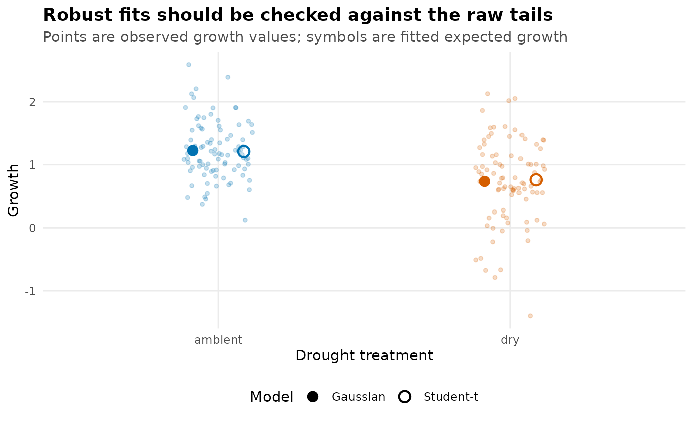
Robust-model check for the seedling example. Faint points show observed growth values; overlaid points compare fitted Gaussian and Student-t expected growth by drought treatment. No interval bars are drawn because this fixture is a raw-data and fitted-point comparison, not an interval summary.

If the mu and sigma conclusions change strongly, the large residuals are not a side detail. They are part of the distributional story and should be reported.

Current boundary

The implemented Student-t path is intentionally narrow:

drmTMB(
  bf(y ~ x1, sigma ~ x2, nu ~ x3),
  family = student(),
  data = dat
)

Student mu random intercepts and independent slopes, a spatial mu term (spatial(1 | id, coords = coords)), and a phylogenetic nu term are implemented, but only at recovery/diagnostic grade: they fit as point estimates and are not coverage-validated, so trust the point estimate, not the interval, and treat them as exploratory. Correlated slopes, labelled covariance blocks, scale (sigma) and shape (nu) random effects, known sampling covariance (meta_V), other structured terms, and bivariate Student-t models are genuinely later phases. Start with this fixed-effect path when you need a robust continuous comparison to a Gaussian location-scale model.

Skew-normal residual asymmetry is a separate fitted fixed-effect family:

drmTMB(
  bf(y ~ x1, sigma ~ x2, nu ~ x3),
  family = skew_normal(),
  data = dat
)

Use this model when the question is residual asymmetry rather than heavy tails. The fitted first slice has density, Gaussian-limit, positive- and negative-skew recovery, false-positive, interval-visibility, and Phase 18 smoke/grid artifact tests. Random effects, known covariance, structured effects, bivariate skew-normal models, residual rho12, aliases such as skew ~ x, and ID-level skewness such as future skew(id) ~ x remain later routes. Gaussian, Student-t, and skew-normal fits answer different residual-distribution questions, so compare them as sensitivity models rather than aliases.