Proportions and success rates • drmTMB

Proportion data are common in ecology and evolution, but the measurement process matters. Some proportions are counts of successes out of known trials: germinated seeds out of seeds planted, infected hosts out of hosts checked, or occupied quadrats out of quadrats surveyed. Other proportions are continuous rates already measured on the unit interval, such as leaf damage, vegetation cover, or the fraction of time an animal spends foraging. This tutorial assumes the location-scale reading pattern from When variance carries signal and extends it to a bounded response.

This article stays inside the currently implemented drmTMB bounded-response surface:

use stats::binomial(link = "logit") for ordinary 0/1 events or counted successes out of known trials with binomial sampling variation only;
use beta_binomial() for counted successes out of known trials when extra-binomial variation is part of the scientific question;
use beta() for continuous proportions strictly inside (0, 1);
use zero_one_beta() for continuous proportions on [0, 1] when exact 0 or 1 values are structural outcomes rather than trial-count outcomes.

The source motivation comes from Nakagawa et al. (2026), who treat overdispersed proportions as part of the same location-scale framework as continuous and count responses. They distinguish discrete proportions from continuous proportions, recommend beta-binomial models for successes out of trials when extra-binomial variation is present, and warn that exact 0 or 1 values in continuous beta responses need explicit zero-one processes rather than being hidden by the model.

Choose The Proportion Route

Start from how the response was measured:

Response	Example	First `drmTMB` family	Boundary status
0/1 event indicator	early NDVI onset, host infected or not, quadrat occupied or not	`stats::binomial(link = "logit")`	rows are ordinary Bernoulli trials; no modelled `sigma`
Counted successes out of trials with ordinary binomial variation	germinated seeds out of planted seeds	`stats::binomial(link = "logit")`	successes can be 0 or all trials through the binomial count process
Counted successes out of trials with extra-binomial variation	germinated seeds out of planted seeds, with tray-to-tray probability scatter	`beta_binomial()`	adds modelled `sigma` for variation beyond binomial sampling
Continuous proportion strictly inside `(0, 1)`	leaf-area damage, vegetation cover, foraging time fraction	`beta()`	exact 0 or 1 is not supported by the strict beta likelihood
Continuous proportion with structural 0 or 1 values	0% disease, 100% cover, complete absence or saturation	`zero_one_beta()`	`zoi` models exact boundary mass; `coi` models exact ones among boundary observations

The distinction is not cosmetic. A denominator-aware model knows that 3 successes out of 6 trials and 30 successes out of 60 trials carry different sampling information. A strict beta model assumes the observation is already a continuous rate and that the boundaries are not part of the observed support. For denominator-aware responses, write cbind(successes, failures). Do not write weights = trials, successes / trials, or cbind(successes, trials): top-level weights are likelihood weights, and the second column of a two-column binomial response is failures, not trial totals.

Plain Binomial Equation And Syntax

Use stats::binomial(link = "logit") when the response is an event probability and ordinary binomial sampling variation is enough:

$\begin{aligned} Y_i \mid n_i, \mu_i &\sim \operatorname{Binomial}(n_i, \mu_i),\\ \operatorname{logit}(\mu_i) &= \beta_0 + \beta_1 \text{canopy}_i + \beta_2 \text{NDVI}_i,\\ E[Y_i / n_i] &= \mu_i,\\ \operatorname{Var}(Y_i / n_i) &= \mu_i(1 - \mu_i) / n_i. \end{aligned}$

For a 0/1 response, $n_i = 1$ :

drmTMB(
  bf(early_onset ~ canopy + ndvi),
  family = stats::binomial(link = "logit"),
  data = onset_data
)

For success counts, keep both the successes and failures:

drmTMB(
  bf(cbind(germinated, failed) ~ treatment + moisture),
  family = stats::binomial(link = "logit"),
  data = seed_trials
)

The fitted mu is the event probability. fitted(fit) and predict(fit, dpar = "mu") return probabilities; multiply by successes_i + failures_i only when the target summary is the expected number of successes.

Here is a small 0/1 event example. Suppose each site is scored for whether a vegetation index crosses an early-season threshold. The model asks how canopy condition and spring NDVI change that event probability:

set.seed(196)
n_onset <- 240
onset_data <- data.frame(
  canopy = factor(
    rep(c("open", "closed"), each = n_onset / 2),
    levels = c("open", "closed")
  ),
  ndvi = as.numeric(scale(runif(n_onset, 0.15, 0.85)))
)

closed <- as.numeric(onset_data$canopy == "closed")
mu_onset <- plogis(-0.85 - 0.35 * closed + 1.10 * onset_data$ndvi)
onset_data$early_onset <- rbinom(n_onset, size = 1, prob = mu_onset)

fit_onset <- drmTMB(
  bf(early_onset ~ canopy + ndvi),
  family = stats::binomial(link = "logit"),
  data = onset_data
)

coef(fit_onset, "mu")
#>  (Intercept) canopyclosed         ndvi 
#>  -0.77939914   0.04603729   0.82133404

Predicted probabilities are already on the response scale:

new_onset <- data.frame(
  canopy = factor(c("open", "closed"), levels = levels(onset_data$canopy)),
  ndvi = c(0, 0)
)

data.frame(
  canopy = new_onset$canopy,
  ndvi = new_onset$ndvi,
  early_onset_probability = predict(fit_onset, newdata = new_onset, dpar = "mu")
)
#>   canopy ndvi early_onset_probability
#> 1   open    0               0.3144494
#> 2 closed    0               0.3244574

The original plain-binomial slice was fixed-effect only. The current R engine also fits ordinary unlabelled mu random intercepts and independent numeric slopes at recovery grade. It still rejects non-logit links, factor responses, proportions with trial weights, correlated or labelled slopes, structured effects, bivariate or mixed responses, and engine = "julia".

Beta-Binomial Equation And Syntax

Use beta_binomial() when the response is still successes out of known trials but the probability varies more than ordinary binomial sampling can explain. The model uses

$\begin{aligned} Y_i \mid n_i, p_i &\sim \operatorname{Binomial}(n_i, p_i),\\ p_i \mid \mu_i, \sigma_i &\sim \operatorname{Beta}(\alpha_i, \beta_i),\\ \operatorname{logit}(\mu_i) &= \beta_0 + \beta_1 \text{sheltered}_i + \beta_2 \text{moisture}_i,\\ \log(\sigma_i) &= \gamma_0 + \gamma_1 \text{sheltered}_i,\\ \phi_i &= 1 / \sigma_i^2,\\ \alpha_i &= \mu_i\phi_i,\\ \beta_i &= (1 - \mu_i)\phi_i,\\ E[Y_i / n_i] &= \mu_i,\\ \operatorname{Var}(Y_i / n_i) &= \frac{\mu_i(1 - \mu_i)(1 + n_i\sigma_i^2)} {n_i(1 + \sigma_i^2)}. \end{aligned}$

The matching drmTMB syntax is:

drmTMB(
  bf(cbind(germinated, failed) ~ treatment + moisture, sigma ~ treatment),
  family = beta_binomial(),
  data = seed_trials
)

If trays, plots, or subjects are repeatedly observed, the first fitted mixed-model slice is an ordinary mu random intercept, optionally paired with an independent numeric mu slope:

drmTMB(
  bf(cbind(germinated, failed) ~ treatment + moisture +
       (1 | tray) + (0 + moisture | tray),
     sigma ~ treatment),
  family = beta_binomial(),
  data = seed_trials
)

The random effects change the logit success-probability predictor. They do not make sigma a random effect, and they do not open correlated slopes or structured bounded-response effects.

Read each parameter before interpreting the fitted model:

Symbol or syntax	Meaning	In the seed-germination example
$Y_i$ , `germinated`	number of successes	seeds that germinated in tray $i$
$n_i$ , `germinated + failed`	known number of trials	viable seeds planted in tray $i$
$\mu_i$ , `mu`	expected success probability	germination probability for a seed in that tray
$\boldsymbol{\beta}_{\mu}$	location coefficients on the logit probability scale	treatment and moisture effects on germination probability
$\sigma_i$ , `sigma`	extra-binomial scale	tray-to-tray probability variation beyond binomial sampling
$\phi_i$	beta precision	`phi_i = 1 / sigma_i^2`, so larger `sigma` means lower precision
$\boldsymbol{\beta}_{\sigma}$	scale coefficients on the log `sigma` scale	treatment effects on extra-binomial variation

If gamma_1 is the sheltered-treatment coefficient, then

$\frac{\sigma_\text{sheltered}}{\sigma_\text{open}} = \exp(\gamma_1), \qquad \frac{\phi_\text{sheltered}}{\phi_\text{open}} = \exp(-2\gamma_1).$

That second ratio reverses direction because $\phi = 1 / \sigma^2$ . In drmTMB, report sigma when you want the direction to mean more or less modelled variation.

Seed Germination Example

Suppose seeds are planted in trays under open and sheltered microsites during a restoration trial. Shelter may increase average germination by reducing heat stress, and it may also make tray outcomes more predictable by buffering microclimate. Each tray has a known number of seeds, so the denominator belongs in the model.

This transparent simulation gives us known structure before fitting:

set.seed(197)
n <- 360
seed_trials <- data.frame(
  treatment = factor(
    rep(c("open", "sheltered"), each = n / 2),
    levels = c("open", "sheltered")
  ),
  moisture = as.numeric(scale(runif(n, 0.1, 0.9))),
  trials = sample(18:32, n, replace = TRUE)
)

sheltered <- as.numeric(seed_trials$treatment == "sheltered")
mu_seed <- plogis(-0.55 + 0.70 * sheltered + 0.45 * seed_trials$moisture)
sigma_seed <- exp(-1.15 - 0.35 * sheltered)
phi_seed <- 1 / sigma_seed^2
tray_probability <- rbeta(
  n,
  shape1 = mu_seed * phi_seed,
  shape2 = (1 - mu_seed) * phi_seed
)

seed_trials$germinated <- rbinom(n, size = seed_trials$trials, prob = tray_probability)
seed_trials$failed <- seed_trials$trials - seed_trials$germinated

head(seed_trials)
#>   treatment    moisture trials germinated failed
#> 1      open  0.79595177     24          4     20
#> 2      open -0.09180242     19          9     10
#> 3      open -1.42799682     29          6     23
#> 4      open -1.54868848     21          3     18
#> 5      open  1.65321214     30         20     10
#> 6      open  0.27586227     20          3     17

Fit the beta-binomial location-scale model:

fit_seed <- drmTMB(
  bf(cbind(germinated, failed) ~ treatment + moisture, sigma ~ treatment),
  family = beta_binomial(),
  data = seed_trials
)

Run diagnostics before interpreting coefficients:

check_drm(fit_seed)
#> <drm_check: 12 checks>
#> ok: 11; notes: 0; warnings: 1; errors: 0
#>                      check  status
#>      optimizer_convergence      ok
#>           optimizer_budget      ok
#>           finite_objective      ok
#>      logsigma_clamp_active      ok
#>             fixed_gradient warning
#>            sdreport_status      ok
#>  hessian_positive_definite      ok
#>     standard_errors_finite      ok
#>   standard_errors_inflated      ok
#>               dropped_rows      ok
#>             positive_scale      ok
#>   fixed_effect_design_size      ok
#>                                                                                   value
#>                                                                                       0
#>                                                 iterations=26; function=37; gradient=27
#>                                                                                   991.7
#>                                                                                    <NA>
#>                                                      max=0.001524; component=beta_mu[1]
#>                                                                                      ok
#>                                                                                    TRUE
#>                                                                  range=[0.03677,0.1156]
#>                                          n_inflated=0; max_se=0.1156; median_se=0.07301
#>                                                                     nobs=360; dropped=0
#>                                                                              min=0.2520
#>  total_mb=0.06031; max_cols=3; largest=mu; largest_class=matrix; largest_density=0.8333
#>                                                                              message
#>                                                        nlminb convergence code is 0.
#>  Optimizer evaluation counts recorded; no eval.max or iter.max control was supplied.
#>                                             Objective and log-likelihood are finite.
#>                                   The log(sigma) clamp is not active at the optimum.
#>         Maximum absolute fixed gradient is > 0.001; largest component is beta_mu[1].
#>                                              TMB::sdreport() completed successfully.
#>                                        sdreport reports a positive-definite Hessian.
#>                                         All fixed-effect standard errors are finite.
#>                   No fixed-effect standard error is inflated relative to the others.
#>                   No rows were dropped by model-frame or known-covariance filtering.
#>                                     All fitted scale values are finite and positive.
#>                          Dense fixed-effect design matrices are modest for this fit.

The mu coefficients describe the log-odds of germination. The sigma coefficients describe extra-binomial variation in the latent tray-level success probability:

coef(fit_seed, "mu")
#>        (Intercept) treatmentsheltered           moisture 
#>         -0.5127846          0.6006894          0.4683619
coef(fit_seed, "sigma")
#>        (Intercept) treatmentsheltered 
#>         -1.1893314         -0.1889193

sigma_ratio <- exp(coef(fit_seed, "sigma")["treatmentsheltered"])
c(
  sigma_ratio_sheltered_vs_open = sigma_ratio,
  precision_ratio_sheltered_vs_open = sigma_ratio^(-2)
)
#>     sigma_ratio_sheltered_vs_open.treatmentsheltered 
#>                                            0.8278533 
#> precision_ratio_sheltered_vs_open.treatmentsheltered 
#>                                            1.4591273

For a response-scale summary, predict the expected success probability and the proportion-level standard deviation for trays with the same number of seeds:

new_seed_trays <- data.frame(
  treatment = factor(c("open", "sheltered"), levels = levels(seed_trials$treatment)),
  moisture = c(0, 0),
  trials = c(24, 24)
)

mu_hat <- predict(fit_seed, newdata = new_seed_trays, dpar = "mu")
sigma_hat <- predict(fit_seed, newdata = new_seed_trays, dpar = "sigma")
prop_var <- mu_hat * (1 - mu_hat) *
  (1 + new_seed_trays$trials * sigma_hat^2) /
  (new_seed_trays$trials * (1 + sigma_hat^2))

data.frame(
  treatment = new_seed_trays$treatment,
  trials = new_seed_trays$trials,
  expected_probability = mu_hat,
  expected_successes = new_seed_trays$trials * mu_hat,
  sigma = sigma_hat,
  phi = 1 / sigma_hat^2,
  proportion_sd = sqrt(prop_var)
)
#>   treatment trials expected_probability expected_successes     sigma      phi
#> 1      open     24             0.374541           8.988983 0.3044247 10.79046
#> 2 sheltered     24             0.521962          12.527089 0.2520190 15.74466
#>   proportion_sd
#> 1     0.1697103
#> 2     0.1570892

This table keeps the two parts of the question separate: expected germination probability and extra-binomial scatter around that probability.

library(ggplot2)

seed_trials$observed_proportion <- seed_trials$germinated / seed_trials$trials
seed_plot_summary <- data.frame(
  treatment = new_seed_trays$treatment,
  expected_probability = mu_hat,
  proportion_sd = sqrt(prop_var)
)
seed_plot_summary$lower <- pmax(
  0,
  seed_plot_summary$expected_probability - seed_plot_summary$proportion_sd
)
seed_plot_summary$upper <- pmin(
  1,
  seed_plot_summary$expected_probability + seed_plot_summary$proportion_sd
)

ggplot(seed_trials, aes(treatment, observed_proportion, colour = treatment)) +
  geom_jitter(width = 0.12, height = 0, alpha = 0.18, size = 0.9) +
  geom_errorbar(
    data = seed_plot_summary,
    aes(
      y = expected_probability,
      ymin = lower,
      ymax = upper
    ),
    width = 0.12,
    linewidth = 0.8
  ) +
  geom_point(data = seed_plot_summary, aes(y = expected_probability), size = 3) +
  scale_colour_manual(values = c("open" = "#0072B2", "sheltered" = "#009E73")) +
  coord_cartesian(ylim = c(0, 1)) +
  labs(
    title = "Denominator-aware proportions can still show raw trays",
    subtitle = "Bars show fitted tray-level scatter, not confidence intervals",
    x = "Microsite treatment",
    y = "Germinated proportion",
    colour = "Treatment"
  ) +
  guides(colour = "none") +
  theme_minimal(base_size = 11) +
  theme(
    panel.grid.minor = element_blank(),
    legend.position = "bottom",
    plot.title = element_text(face = "bold"),
    plot.subtitle = element_text(colour = "grey30")
  )

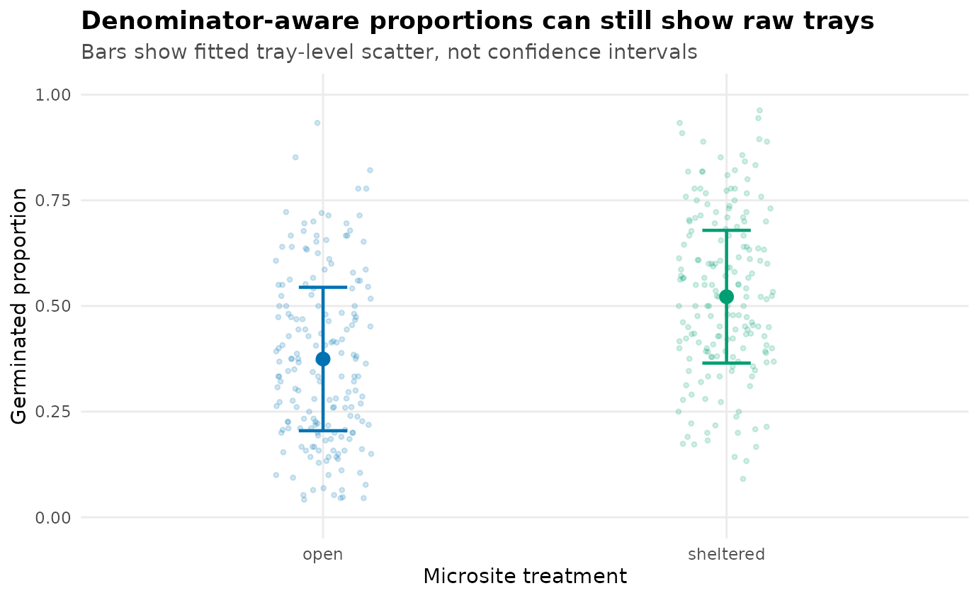
Jittered point plot of observed germination proportions for open and sheltered trays. Overlaid larger points show fitted expected probabilities, and vertical bars show one fitted proportion-level standard deviation for each treatment.

Beta-binomial tray summary for the seed-germination example. Faint points are observed tray proportions; overlaid points are fitted expected germination probabilities; vertical bars show plus or minus one fitted proportion-level standard deviation, not confidence intervals.

Strict Continuous Proportions

Use beta() when the response is a continuous proportion strictly inside the open interval. For example, vegetation cover measured from image analysis may record 0.03, 0.41, or 0.82 rather than successes out of a known number of quadrats. The beta model uses

$\begin{aligned} Y_i \mid \mu_i, \sigma_i &\sim \operatorname{Beta}(\alpha_i, \beta_i),\\ \operatorname{logit}(\mu_i) &= \beta_0 + \beta_1 \text{grazed}_i + \beta_2 \text{moisture}_i,\\ \log(\sigma_i) &= \gamma_0 + \gamma_1 \text{grazed}_i,\\ \phi_i &= 1 / \sigma_i^2,\\ \operatorname{Var}(Y_i) &= \frac{\mu_i(1 - \mu_i)\sigma_i^2}{1 + \sigma_i^2}. \end{aligned}$

The fitted syntax is the same one-formula-per-parameter pattern:

drmTMB(
  bf(cover ~ grazing + moisture, sigma ~ grazing),
  family = beta(),
  data = cover_data
)

A small transparent example:

set.seed(198)
n_cover <- 300
cover_data <- data.frame(
  grazing = factor(
    rep(c("ungrazed", "grazed"), each = n_cover / 2),
    levels = c("ungrazed", "grazed")
  ),
  moisture = as.numeric(scale(runif(n_cover, 0.05, 0.95)))
)

grazed <- as.numeric(cover_data$grazing == "grazed")
mu_cover <- plogis(0.35 - 0.75 * grazed + 0.35 * cover_data$moisture)
sigma_cover <- exp(-1.10 + 0.45 * grazed)
phi_cover <- 1 / sigma_cover^2
cover_data$cover <- rbeta(
  n_cover,
  shape1 = mu_cover * phi_cover,
  shape2 = (1 - mu_cover) * phi_cover
)

fit_cover <- drmTMB(
  bf(cover ~ grazing + moisture, sigma ~ grazing),
  family = beta(),
  data = cover_data
)

check_drm(fit_cover)
#> <drm_check: 12 checks>
#> ok: 12; notes: 0; warnings: 0; errors: 0
#>                      check status
#>      optimizer_convergence     ok
#>           optimizer_budget     ok
#>           finite_objective     ok
#>      logsigma_clamp_active     ok
#>             fixed_gradient     ok
#>            sdreport_status     ok
#>  hessian_positive_definite     ok
#>     standard_errors_finite     ok
#>   standard_errors_inflated     ok
#>               dropped_rows     ok
#>             positive_scale     ok
#>   fixed_effect_design_size     ok
#>                                                                                   value
#>                                                                                       0
#>                                                 iterations=28; function=38; gradient=29
#>                                                                                  -93.38
#>                                                                                    <NA>
#>                                                     max=0.0007696; component=beta_mu[1]
#>                                                                                      ok
#>                                                                                    TRUE
#>                                                                 range=[0.04484,0.09263]
#>                                         n_inflated=0; max_se=0.09263; median_se=0.05555
#>                                                                     nobs=300; dropped=0
#>                                                                              min=0.3531
#>  total_mb=0.05065; max_cols=3; largest=mu; largest_class=matrix; largest_density=0.8333
#>                                                                              message
#>                                                        nlminb convergence code is 0.
#>  Optimizer evaluation counts recorded; no eval.max or iter.max control was supplied.
#>                                             Objective and log-likelihood are finite.
#>                                   The log(sigma) clamp is not active at the optimum.
#>        Maximum absolute fixed gradient is <= 0.001; largest component is beta_mu[1].
#>                                              TMB::sdreport() completed successfully.
#>                                        sdreport reports a positive-definite Hessian.
#>                                         All fixed-effect standard errors are finite.
#>                   No fixed-effect standard error is inflated relative to the others.
#>                   No rows were dropped by model-frame or known-covariance filtering.
#>                                     All fitted scale values are finite and positive.
#>                          Dense fixed-effect design matrices are modest for this fit.

Here, grazing changes both expected cover and the variation of cover among sampling units:

coef(fit_cover, "mu")
#>   (Intercept) grazinggrazed      moisture 
#>     0.3732632    -0.7837726     0.3590303
coef(fit_cover, "sigma")
#>   (Intercept) grazinggrazed 
#>    -1.0410602     0.3442394

new_cover <- data.frame(
  grazing = factor(c("ungrazed", "grazed"), levels = levels(cover_data$grazing)),
  moisture = c(0, 0)
)

mu_cover_hat <- predict(fit_cover, newdata = new_cover, dpar = "mu")
sigma_cover_hat <- predict(fit_cover, newdata = new_cover, dpar = "sigma")

data.frame(
  grazing = new_cover$grazing,
  expected_cover = mu_cover_hat,
  sigma = sigma_cover_hat,
  phi = 1 / sigma_cover_hat^2,
  cover_sd = sqrt(
    mu_cover_hat * (1 - mu_cover_hat) *
      sigma_cover_hat^2 / (1 + sigma_cover_hat^2)
  )
)
#>    grazing expected_cover     sigma      phi  cover_sd
#> 1 ungrazed      0.5922473 0.3530802 8.021459 0.1636107
#> 2   grazed      0.3987900 0.4981666 4.029497 0.2183348

Do not use this strict beta route if the observed response includes exact 0 or 1 values. A sprayed plot with 0% damage or a quadrat with 100% cover is a boundary-generating process, not an interior beta observation. Use zero_one_beta() when those endpoints are structural outcomes.

Continuous Proportions With Exact Boundaries

Use zero_one_beta() when the response is a continuous proportion on [0, 1] and exact 0 or 1 values are generated by a separate boundary process. The interior observations still use the beta mean-scale model. The two extra probability formulas describe the boundary process:

$\begin{aligned} \Pr(Y_i = 0) &= zoi_i(1 - coi_i),\\ \Pr(Y_i = 1) &= zoi_i coi_i,\\ \Pr(0 < Y_i < 1) &= 1 - zoi_i,\\ \operatorname{logit}(\mu_i) &= \beta_0 + \beta_1 \text{grazed}_i,\\ \log(\sigma_i) &= \gamma_0 + \gamma_1 \text{grazed}_i,\\ \operatorname{logit}(zoi_i) &= \delta_0 + \delta_1 \text{drought}_i,\\ \operatorname{logit}(coi_i) &= \kappa_0 + \kappa_1 \text{canopy}_i. \end{aligned}$

drmTMB(
  bf(cover ~ grazing, sigma ~ grazing, zoi ~ drought, coi ~ canopy),
  family = zero_one_beta(),
  data = cover_data
)

predict(fit, dpar = "mu") describes the mean among interior observations. predict(fit, dpar = "zoi") is the probability of an exact boundary outcome, and predict(fit, dpar = "coi") is the probability that a boundary outcome is exactly 1. fitted(fit) returns the unconditional mean (1 - zoi) * mu + zoi * coi, which is usually the response-scale summary an applied reader expects.

Current Boundary

The implemented bounded-response path is univariate. Use stats::binomial(link = "logit") for ordinary fixed-effect event probability models, beta_binomial() for overdispersed counted successes and failures, beta() for a single continuous proportion strictly between 0 and 1, and zero_one_beta() for a single continuous proportion with structural exact 0 or 1 values. beta() and beta_binomial() support ordinary unlabelled mu random intercepts and independent numeric slopes as first mixed-model slices:

drmTMB(
  bf(cbind(successes, failures) ~ treatment + dose +
       (1 | id) + (0 + dose | id),
     sigma ~ treatment),
  family = beta_binomial(),
  data = dat
)

drmTMB(
  bf(proportion ~ treatment + dose + (1 | id) + (0 + dose | id),
     sigma ~ treatment),
  family = beta(),
  data = dat
)

Do not teach the following as fitted proportion examples yet:

correlated random slopes, labelled covariance blocks, or random effects in sigma, zoi, or coi;
sd(group) ~ ... random-effect scale models;
meta_V(V = V), or deprecated meta_known_V(V = V) for compatibility, with beta or beta-binomial responses;
phylo(), spatial(), animal(), or relmat() bounded-response models, with one exception: beta() already accepts a single unlabelled animal() term – an intercept or one-slope on mu, or an intercept on sigma, one endpoint at a time – but only at recovery grade (trust the point estimate, not the interval), so it is held back here on tier grounds, not for want of likelihood code;
bivariate or mixed-response bounded models such as family = c(beta(), gaussian());
ordered beta or beta-binomial zero-inflation;
denominator shorthand such as successes / trials, weights = trials, or cbind(successes, trials) as a replacement for cbind(successes, failures).

Most of those are useful future routes that still need likelihood code, simulation recovery, diagnostics, and source-map evidence before they become tutorial syntax.