When variance carries signal, Part 1: location-scale models • drmTMB

This tutorial starts with a biological question: do two habitats differ only in mean growth, or does one habitat also make growth less predictable? In a Gaussian location-scale model, the location part models the expected response mu, while the scale part models the residual standard deviation sigma. That residual scale is not just a nuisance parameter; it can be the scientific answer when the question is about individual variability, predictability, or remaining heterogeneity after the mean model is accounted for.

This is Part 1 of a two-article sequence. It models the response mean mu and the residual standard deviation sigma. Continue to Part 2: location-scale-scale models when a predictor should model the standard deviation of a latent group or phylogenetic random effect through sd().

Read this after you have fit a first model in Distributional regression with drmTMB and confirmed Gaussian is the right family in Choosing response families; this tutorial goes deeper into interpreting mu and sigma once that choice is made.

If you are fitting your first model, start with the worked growth example, then return to the syntax overview below when you want to adapt the formula.

The core Gaussian location-scale route supports fixed effects, optional random effects in the location formula, and residual-scale random intercepts and independent random slopes in the sigma formula. The same pattern is used throughout the documentation: write the model symbolically first, show the matching R syntax, fit the model, and interpret the fitted output.

Model equations and matching R syntax

For Gaussian location-scale regression, each estimated parameter has its own linear predictor:

$\begin{aligned} y_i \mid \mu_i, \sigma_i &\sim \operatorname{Normal}(\mu_i, \sigma_i^2),\\ \mu_i &= \mathbf{x}_i^{\mathsf T}\boldsymbol\beta,\\ \log(\sigma_i) &= \mathbf{z}_i^{\mathsf T}\boldsymbol\gamma. \end{aligned}$

The matching syntax is:

drmTMB(
  bf(y ~ x, sigma ~ z),
  family = gaussian(),
  data = dat
)

The location formula defines the design matrix for beta; the scale formula defines the design matrix for gamma. The log link keeps the fitted residual SD positive.

Quantity	R source	Interpretation
`mu_i`	`y ~ x`	expected response
`beta`	`coef(fit, "mu")`	additive effects on the expected response
`sigma_i`	`sigma ~ z`	residual SD around the fitted mean
`gamma`	`coef(fit, "sigma")`	effects on log residual SD

Grouped effects do not change the meaning of sigma

A random intercept in the location model adds among-group variation in expected responses:

$\mu_{ij} = \mathbf{x}_{ij}^{\mathsf T}\boldsymbol\beta + b_j, \qquad b_j \sim \operatorname{Normal}(0,sd_{\mu,group}^2).$

drmTMB(
  bf(y ~ x + (1 | group), sigma ~ z),
  family = gaussian(),
  data = dat
)

Here sd_mu_group is the SD of group-level mean deviations. It is not the residual SD sigma. A random effect inside the sigma formula asks a third question: do groups differ in their residual variability?

drmTMB(
  bf(y ~ x + (1 | group), sigma ~ z + (1 | group)),
  family = gaussian(),
  data = dat
)

More elaborate ordinary intercept-slope blocks and their covariance output are documented in Which scale are you modelling? and Structural dependence. To model predictors of the group-level SD itself, continue to Part 2: location-scale-scale models.

Interpret sigma on the SD or variance scale

Because log(sigma_i) = z_i^T gamma, exponentiating a scale coefficient gives an SD ratio. If gamma_temperature = 0.3, then a one-unit temperature increase multiplies residual SD by exp(0.3) = 1.35. Squaring the ratio gives the residual-variance ratio, exp(2 * 0.3) = 1.82.

Formula component	Report	Biological reading
`growth ~ temperature`	`beta_temperature`	additive change in expected growth
`sigma ~ temperature`	`exp(gamma_temperature)`	residual-SD ratio per temperature unit
`(0 + temperature \| population)` in `mu`	random-slope SD	variation among population-specific mean slopes
`sigma ~ (0 + temperature \| population)`	residual-scale random-slope SD	variation among population-specific log-SD slopes

Name the measured response and model component before stating a biological conclusion. “Temperature-dependent variability” is ambiguous until the reader knows whether the model changed residual sigma, a mean random-slope SD, or a random effect inside sigma.

Worked example: growth mean and predictability

Suppose an ecologist measures juvenile growth in two habitats and records the temperature at each observation. The location question is whether mean growth differs between habitats and changes with temperature. The scale question is whether residual growth variability differs between habitats after accounting for those mean effects.

For this example, the fitted model is:

$\begin{aligned} \text{growth}_i &\sim \operatorname{Normal}(\mu_i, \sigma_i^2), \\ \mu_i &= \beta_0 + \beta_1 \mathbb{1}(\text{habitat}_i = \text{grassland}) + \beta_2 \text{temperature}_i, \\ \log(\sigma_i) &= \gamma_0 + \gamma_1 \mathbb{1}(\text{habitat}_i = \text{grassland}). \end{aligned}$

The matching drmTMB syntax is:

drmTMB(
  drm_formula(growth ~ habitat + temperature, sigma ~ habitat),
  family = gaussian(),
  data = dat
)

The code below simulates one dataset with the same structure. Simulated data keep the vignette small and reproducible; a real analysis would replace this block with field or laboratory measurements.

set.seed(42)
n <- 240
dat <- data.frame(
  habitat = factor(rep(c("forest", "grassland"), each = n / 2)),
  temperature = rnorm(n)
)

mu <- 8 + 1.2 * (dat$habitat == "grassland") + 0.6 * dat$temperature
sigma_true <- exp(log(0.6) + 0.55 * (dat$habitat == "grassland"))
dat$growth <- rnorm(n, mean = mu, sd = sigma_true)

Fit the location-scale model:

fit_growth <- drmTMB(
  drm_formula(growth ~ habitat + temperature, sigma ~ habitat),
  family = gaussian(),
  data = dat
)

Before interpreting coefficients, check the fitted object:

check_drm(fit_growth)
#> <drm_check: 12 checks>
#> ok: 12; notes: 0; warnings: 0; errors: 0
#>                      check status
#>      optimizer_convergence     ok
#>           optimizer_budget     ok
#>           finite_objective     ok
#>      logsigma_clamp_active     ok
#>             fixed_gradient     ok
#>            sdreport_status     ok
#>  hessian_positive_definite     ok
#>     standard_errors_finite     ok
#>   standard_errors_inflated     ok
#>               dropped_rows     ok
#>             positive_scale     ok
#>   fixed_effect_design_size     ok
#>                                                                                   value
#>                                                                                       0
#>                                                 iterations=19; function=33; gradient=19
#>                                                                                   279.3
#>                                                                                    <NA>
#>                                                  max=0.0008192; component=beta_sigma[2]
#>                                                                                      ok
#>                                                                                    TRUE
#>                                                                  range=[0.04551,0.1102]
#>                                          n_inflated=0; max_se=0.1102; median_se=0.06466
#>                                                                     nobs=240; dropped=0
#>                                                                              min=0.5633
#>  total_mb=0.04107; max_cols=3; largest=mu; largest_class=matrix; largest_density=0.8333
#>                                                                              message
#>                                                        nlminb convergence code is 0.
#>  Optimizer evaluation counts recorded; no eval.max or iter.max control was supplied.
#>                                             Objective and log-likelihood are finite.
#>                                   The log(sigma) clamp is not active at the optimum.
#>     Maximum absolute fixed gradient is <= 0.001; largest component is beta_sigma[2].
#>                                              TMB::sdreport() completed successfully.
#>                                        sdreport reports a positive-definite Hessian.
#>                                         All fixed-effect standard errors are finite.
#>                   No fixed-effect standard error is inflated relative to the others.
#>                   No rows were dropped by model-frame or known-covariance filtering.
#>                                     All fitted scale values are finite and positive.
#>                          Dense fixed-effect design matrices are modest for this fit.

The interval target inventory is part of the same interpretation gate. For this fixed-effect example, every coefficient is a direct profile target:

profile_targets(fit_growth)[
  ,
  c("parm", "estimate", "profile_ready", "profile_note")
]
#>                           parm   estimate profile_ready profile_note
#> 1         fixef:mu:(Intercept)  7.9948246          TRUE        ready
#> 2    fixef:mu:habitatgrassland  1.2068575          TRUE        ready
#> 3         fixef:mu:temperature  0.5745448          TRUE        ready
#> 4      fixef:sigma:(Intercept) -0.5740134          TRUE        ready
#> 5 fixef:sigma:habitatgrassland  0.6376342          TRUE        ready

Now print the coefficient table:

summary(fit_growth)
#> <summary.drmTMB>
#> estimator: ML
#>                          estimate  std_error
#> mu:(Intercept)          7.9948246 0.05143610
#> mu:habitatgrassland     1.2068575 0.11021142
#> mu:temperature          0.5745448 0.04550947
#> sigma:(Intercept)      -0.5740134 0.06466108
#> sigma:habitatgrassland  0.6376342 0.09160089
#> Distributional, random-effect, scale, and correlation parameters:
#>                         component  dpar         term  estimate   minimum
#> fitted:sigma distributional-scale sigma fitted range 0.8144743 0.5632603
#>               maximum    scale
#> fitted:sigma 1.065688 response
#> logLik: -279.3
#> convergence: 0

How to read this output:

Rows beginning with mu: are mean-growth effects on the response scale. For example, mu:temperature is the expected change in mean growth for a one-unit increase in temperature.
Rows beginning with sigma: are log-residual-standard-deviation effects. For example, sigma:habitatgrassland is not an additive change in growth; it is a log-scale change in residual variability.
Exponentiating a sigma coefficient gives the multiplicative change in residual standard deviation.

sigma_habitat <- coef(fit_growth, "sigma")["habitatgrassland"]
data.frame(
  coefficient = sigma_habitat,
  residual_sd_ratio = exp(sigma_habitat),
  residual_variance_ratio = exp(2 * sigma_habitat)
)
#>                  coefficient residual_sd_ratio residual_variance_ratio
#> habitatgrassland   0.6376342             1.892                3.579662

In this fitted example, exp(sigma:habitatgrassland) is the estimated ratio of grassland residual SD to forest residual SD. A value near 2 means that grassland has about twice the residual SD of forest after accounting for mean habitat and temperature effects. Because residual variance is SD squared, the same fitted coefficient implies about four times the residual variance.

It is often clearer to report the fitted residual SDs and variances directly:

newdat <- data.frame(
  habitat = factor(c("forest", "grassland"), levels = levels(dat$habitat)),
  temperature = 0
)

growth_report <- data.frame(
  habitat = newdat$habitat,
  fitted_mean_growth = predict(fit_growth, newdata = newdat, dpar = "mu"),
  fitted_residual_sd = predict(fit_growth, newdata = newdat, dpar = "sigma")
)
growth_report$fitted_residual_variance <- growth_report$fitted_residual_sd^2
growth_report
#>     habitat fitted_mean_growth fitted_residual_sd fitted_residual_variance
#> 1    forest           7.994825          0.5632603                0.3172622
#> 2 grassland           9.201682          1.0656882                1.1356914

This table maps the model back to the scientific question. The mean column summarises the location model. The residual SD column summarises the scale model in the units of growth. The residual variance column is the variance-facing version of the same fitted Gaussian scale model.

The fitted mean can be checked against the raw response pattern. Here the points are observed growth values; the fitted lines and ribbons come from predict_parameters() on an explicit temperature-by-habitat grid:

growth_mu_grid <- prediction_grid(
  fit_growth,
  focal = c("temperature", "habitat"),
  at = list(
    temperature = seq(
      min(dat$temperature),
      max(dat$temperature),
      length.out = 80
    )
  )
)

growth_mu_surface <- predict_parameters(
  fit_growth,
  newdata = growth_mu_grid,
  dpar = "mu",
  conf.int = TRUE
)

unique(growth_mu_surface[, c(
  "dpar",
  "conf.status",
  "interval_source",
  "conf.level"
)])
#>   dpar conf.status interval_source conf.level
#> 1   mu        wald            wald       0.95

if (requireNamespace("ggplot2", quietly = TRUE)) {
  ggplot2::ggplot(
    dat,
    ggplot2::aes(x = temperature, y = growth, colour = habitat)
  ) +
    ggplot2::geom_point(alpha = 0.38, size = 1.25) +
    ggplot2::geom_ribbon(
      data = growth_mu_surface,
      ggplot2::aes(
        x = temperature,
        ymin = conf.low,
        ymax = conf.high,
        fill = habitat
      ),
      inherit.aes = FALSE,
      alpha = 0.18,
      colour = NA
    ) +
    ggplot2::geom_line(
      data = growth_mu_surface,
      ggplot2::aes(y = estimate),
      linewidth = 0.85
    ) +
    location_scale_habitat_scales() +
    ggplot2::labs(
      title = "Mean growth and observed scatter",
      subtitle = "Points are raw growth; ribbons are 95% Wald bands for mu",
      x = "Temperature",
      y = "Growth",
      colour = "Habitat",
      fill = "Habitat"
    ) +
    location_scale_theme() +
    ggplot2::guides(fill = "none")
}

Scatterplot of simulated growth over temperature for forest and grassland habitats, with fitted mean growth lines and 95 percent Wald confidence bands for each habitat.

Raw growth observations and fitted response-scale mu surfaces for the Gaussian location-scale example; ribbons are 95% Wald confidence bands from predict_parameters().

The scale model is a different display. Do not put raw growth points on the sigma axis; plot the fitted residual SD and name the interval source:

growth_sigma_grid <- prediction_grid(
  fit_growth,
  focal = "habitat",
  condition = list(temperature = 0)
)

growth_sigma_surface <- predict_parameters(
  fit_growth,
  newdata = growth_sigma_grid,
  dpar = "sigma",
  conf.int = TRUE
)

unique(growth_sigma_surface[, c(
  "dpar",
  "conf.status",
  "interval_source",
  "conf.level"
)])
#>    dpar conf.status interval_source conf.level
#> 1 sigma        wald            wald       0.95

if (requireNamespace("ggplot2", quietly = TRUE)) {
  ggplot2::ggplot(
    growth_sigma_surface,
    ggplot2::aes(x = estimate, y = habitat, colour = habitat)
  ) +
    ggplot2::geom_segment(
      ggplot2::aes(x = conf.low, xend = conf.high, yend = habitat),
      linewidth = 0.8
    ) +
    ggplot2::geom_point(size = 2.8) +
    location_scale_habitat_scales() +
    ggplot2::labs(
      title = "Residual SD differs by habitat",
      subtitle = "Points are fitted sigma values; bars are 95% Wald intervals",
      x = "Fitted residual SD (sigma)",
      y = NULL,
      colour = "Habitat"
    ) +
    location_scale_theme() +
    ggplot2::guides(colour = "none")
}
#> Warning: No shared levels found between `names(values)` of the manual scale and the
#> data's fill values.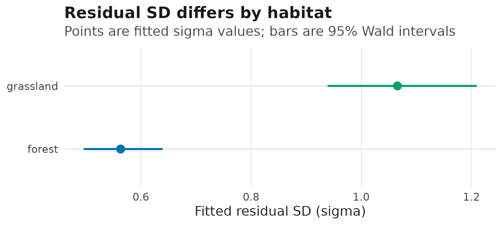

Horizontal point interval plot comparing fitted residual standard deviation for forest and grassland habitats at temperature zero, with 95 percent Wald confidence intervals.

Fitted residual standard deviations by habitat at average temperature; horizontal intervals are 95% Wald confidence intervals requested from predict_parameters().

The compact translation table below is the reporting layer Pat should be able to read without returning to the equations:

growth_translation <- data.frame(
  model_piece = c(
    "fixed mean slope",
    "fixed residual-SD contrast",
    "fixed residual-variance contrast"
  ),
  fitted_term = c(
    "mu:temperature",
    "exp(sigma:habitatgrassland)",
    "exp(2 * sigma:habitatgrassland)"
  ),
  response_scale_value = c(
    unname(coef(fit_growth, "mu")["temperature"]),
    unname(exp(sigma_habitat)),
    unname(exp(2 * sigma_habitat))
  ),
  interpretation = c(
    "mean growth change per one-unit temperature increase",
    "grassland residual SD divided by forest residual SD",
    "grassland residual variance divided by forest residual variance"
  )
)
growth_translation$response_scale_value <-
  round(growth_translation$response_scale_value, 3)
growth_translation
#>                        model_piece                     fitted_term
#> 1                 fixed mean slope                  mu:temperature
#> 2       fixed residual-SD contrast     exp(sigma:habitatgrassland)
#> 3 fixed residual-variance contrast exp(2 * sigma:habitatgrassland)
#>   response_scale_value
#> 1                0.575
#> 2                1.892
#> 3                3.580
#>                                                    interpretation
#> 1            mean growth change per one-unit temperature increase
#> 2             grassland residual SD divided by forest residual SD
#> 3 grassland residual variance divided by forest residual variance

A report can now say three concrete things. Mean growth increases by the fitted mu:temperature slope for each one-unit temperature increase. Grassland has the fitted residual-SD ratio in the second row after accounting for mean habitat and temperature effects. Because Gaussian variance is sigma^2, the residual variance contrast is the third row. If that third row is larger than one, individual growth is less predictable in grassland.

The same reporting discipline carries over to hierarchical versions of the question:

If the biological question is…	Fit this kind of term	Report this quantity	Check before reporting
Do populations differ in thermal plasticity?	`(0 + temperature \| population)` or `(1 + temperature \| population)` in the `mu` formula	the random-slope SD, in growth-per-temperature units	`check_drm(fit)` and the matching `sd:mu:...temperature...` row in `profile_targets(fit)`
Do high-baseline populations also have steeper thermal reaction norms?	`(1 + temperature \| population)` in the `mu` formula	the random-slope SD, and when the correlated block is fitted, the group-level intercept-slope correlation from `corpairs(fit, class = "mean-slope")`	`check_drm(fit)`, the matching `sd:mu:...temperature...` row, and the fitted correlation row in `profile_targets(fit)`
Does predictability change with temperature?	`sigma ~ temperature`	`exp(gamma_temperature)` as the residual-SD ratio, and `exp(2 * gamma_temperature)` when the paper talks about variance	`check_drm(fit)` and the `fixef:sigma:temperature` row in `profile_targets(fit)`
Do habitats differ in among-population variation?	`(1 \| population)` plus `sd(population) ~ habitat`	`exp(alpha_habitat)` as the ratio of among-population SDs	`check_drm(fit)` and the `fixef:sd(population):...` row in `profile_targets(fit)`

These three rows answer different biological questions. sigma ~ temperature models residual variation among observations. (0 + temperature | population) models population-to-population differences in the mean slope. sd(population) ~ habitat models the size of among-population mean differences.

Curved responses and interactions

Quadratic terms and interactions can appear in either formula:

fit_curve <- drmTMB(
  bf(
    growth ~ habitat * temperature + I(temperature^2),
    sigma ~ I(temperature^2)
  ),
  family = gaussian(),
  data = dat
)

A linear coefficient is only a local slope when its model also contains a quadratic term or interaction. Interpret the fitted curve at biologically meaningful predictor values rather than reading that coefficient alone:

curve_grid <- expand.grid(
  habitat = c("forest", "grassland"),
  temperature = c(-1.5, 0, 1.5)
)

data.frame(
  curve_grid,
  mu = predict(fit_curve, newdata = curve_grid, dpar = "mu"),
  sigma = predict(fit_curve, newdata = curve_grid, dpar = "sigma")
)

If the sigma formula is omitted, drmTMB fits one intercept-only residual SD. Use that simpler model only when a common residual SD is scientifically and diagnostically adequate.

Where to continue

Use Part 2: location-scale-scale models when predictors model a grouped or phylogenetic random-effect SD through sd().
Use Mean effects and residual heterogeneity for Gaussian meta-analysis with known sampling covariance through meta_V(V = V).
Use Changing residual coupling with rho12 for two responses and predictor-dependent residual correlation.
Use Structural dependence for phylo(), animal(), spatial(), and relmat().

Current implementation boundaries

This article documents the univariate Gaussian mu and sigma route.
Random intercepts, independent slopes, and ordinary correlated intercept-slope blocks are available in mu; sigma supports its documented random-intercept and random-slope slices.
Scale coefficients use a log-SD link. Exponentiate once for an SD ratio and twice in the exponent for a variance ratio.
Missing rows are removed when variables used by either formula are missing.
A fitted optimizer code is not enough: run check_drm(), inspect gradient and Hessian diagnostics, and use What can I trust? before widening the claim.
sigma is not a group random-effect SD. Use Part 2 for the separate sd(group) ~ predictors grammar.