This article shows the plot grammar that Phase 18 simulation reports should use before broad simulation grids are advertised as evidence. It is a display contract, not a final result report. It assumes you are already tracking a slice in the implementation map and need its recovery evidence plotted before closing that slice out. The small tables below are illustrative fixtures that mimic the columns a real simulation summary should carry.
Simulation figures should answer the same reader questions across continuous, proportion, count, and meta-analysis examples:
- Does the estimator recover the truth without important bias?
- How large is the error, measured by RMSE?
- Do interval procedures cover at the advertised rate?
- Does power increase under the intended effect?
- How often do fits converge, hit boundaries, warn, or fail?
- How much runtime does each surface require?
library(ggplot2)

theme_sim_grammar <- function() {
  theme_minimal(base_size = 11) +
    theme(
      panel.grid.minor = element_blank(),
      panel.grid.major.y = element_blank(),
      plot.title.position = "plot",
      plot.title = element_text(face = "bold"),
      plot.subtitle = element_text(colour = "grey30", lineheight = 1.05),
      strip.text = element_text(face = "bold"),
      legend.position = "bottom",
      plot.margin = margin(6, 10, 12, 6)
    )
}

surface_palette <- c(
  "Gaussian location-scale" = "#0072B2",
  "Proportion" = "#009E73",
  "Count" = "#D55E00",
  "Meta-analysis" = "#CC79A7"
)

surface_levels <- names(surface_palette)
surface_facet_labels <- c(
  "Gaussian location-scale" = "Gaussian\nlocation-scale",
  "Proportion" = "Proportion",
  "Count" = "Count",
  "Meta-analysis" = "Meta-analysis"
)
estimand_display_labels <- c(
  "beta_x" = "beta_x",
  "sigma" = "sigma",
  "sd_group" = "sd(group)",
  "rho12" = "rho12"
)
Bias and RMSE
Bias and RMSE should be plotted beside the estimand. A single average
across all parameters hides the distinction between fixed effects,
residual scale, random-effect SDs, and residual correlation
rho12.
set.seed(20260519)
ggplot(accuracy_replicate_display, aes(error, estimand)) +
  geom_vline(xintercept = 0, linetype = "dotted", colour = "grey55") +
  geom_violin(
    aes(
      fill = surface
    ),
    width = 0.62,
    alpha = 0.16,
    colour = NA,
    scale = "width",
    trim = FALSE
  ) +
  geom_point(
    aes(colour = surface),
    position = position_jitter(height = 0.05, width = 0),
    alpha = 0.22,
    size = 0.65,
    show.legend = FALSE
  ) +
  geom_errorbar(
    data = accuracy_summary,
    aes(
      xmin = bias_low,
      xmax = bias_high,
      y = estimand,
      colour = surface
    ),
    inherit.aes = FALSE,
    orientation = "y",
    width = 0.16,
    linewidth = 0.65,
    na.rm = TRUE
  ) +
  geom_point(
    data = accuracy_summary,
    aes(bias, estimand, colour = surface),
    size = 2.4,
    na.rm = TRUE
  ) +
  geom_text(
    data = accuracy_missing,
    aes(
      x = bias_missing_x,
      y = estimand,
      label = missing_label
    ),
    colour = "grey55",
    size = 2.25,
    lineheight = 0.9,
    hjust = 0,
    inherit.aes = FALSE
  ) +
  facet_wrap(
    ~surface,
    nrow = 1,
    labeller = labeller(surface = as_labeller(surface_facet_labels))
  ) +
  scale_colour_manual(values = surface_palette, drop = FALSE) +
  scale_fill_manual(values = surface_palette, drop = FALSE) +
  labs(
    title = "Bias displays should show replicate-level error",
    subtitle = "Faint dots sample fixture replicate errors; points/bars show mean bias with 95% MCSE",
    x = "Estimate minus truth",
    y = NULL,
    colour = "Surface"
  ) +
  scale_x_continuous(
    breaks = c(-0.5, 0, 0.5),
    labels = c("-0.5", "0.0", "0.5")
  ) +
  coord_cartesian(xlim = c(-0.72, 0.72)) +
  scale_y_discrete(labels = estimand_display_labels) +
  guides(colour = "none", fill = "none") +
  theme_sim_grammar()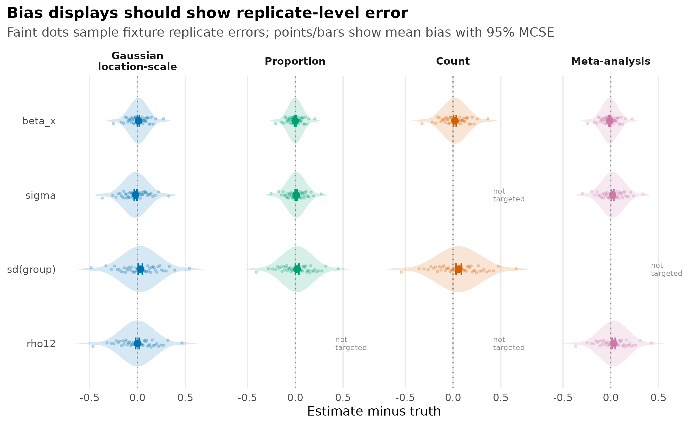
Bias fixture showing sampled replicate-level signed errors, aggregate mean-bias points, and 95% Monte Carlo standard-error intervals by simulation surface.
ggplot(accuracy_summary, aes(rmse, estimand, colour = surface)) +
  geom_errorbar(
    aes(
      xmin = rmse_low,
      xmax = rmse_high
    ),
    orientation = "y",
    width = 0.15,
    linewidth = 0.9,
    alpha = 0.9,
    na.rm = TRUE
  ) +
  geom_point(size = 2.4, na.rm = TRUE) +
  geom_text(
    data = accuracy_missing,
    aes(
      x = rmse_missing_x,
      y = estimand,
      label = missing_label
    ),
    colour = "grey55",
    size = 2.25,
    lineheight = 0.9,
    hjust = 0,
    inherit.aes = FALSE
  ) +
  facet_wrap(
    ~surface,
    nrow = 2,
    labeller = labeller(surface = as_labeller(surface_facet_labels))
  ) +
  scale_colour_manual(values = surface_palette, drop = FALSE) +
  labs(
    title = "RMSE needs its own uncertainty display",
    subtitle = "Facets are surfaces; points and bars are RMSE and 95% MCSE intervals for each estimand",
    x = "Root mean-square error",
    y = NULL,
    colour = "Surface"
  ) +
  scale_x_continuous(
    breaks = c(0, 0.10, 0.20),
    limits = c(0, 0.31),
    expand = expansion(mult = c(0.01, 0.04))
  ) +
  scale_y_discrete(labels = estimand_display_labels) +
  guides(colour = "none") +
  theme_sim_grammar()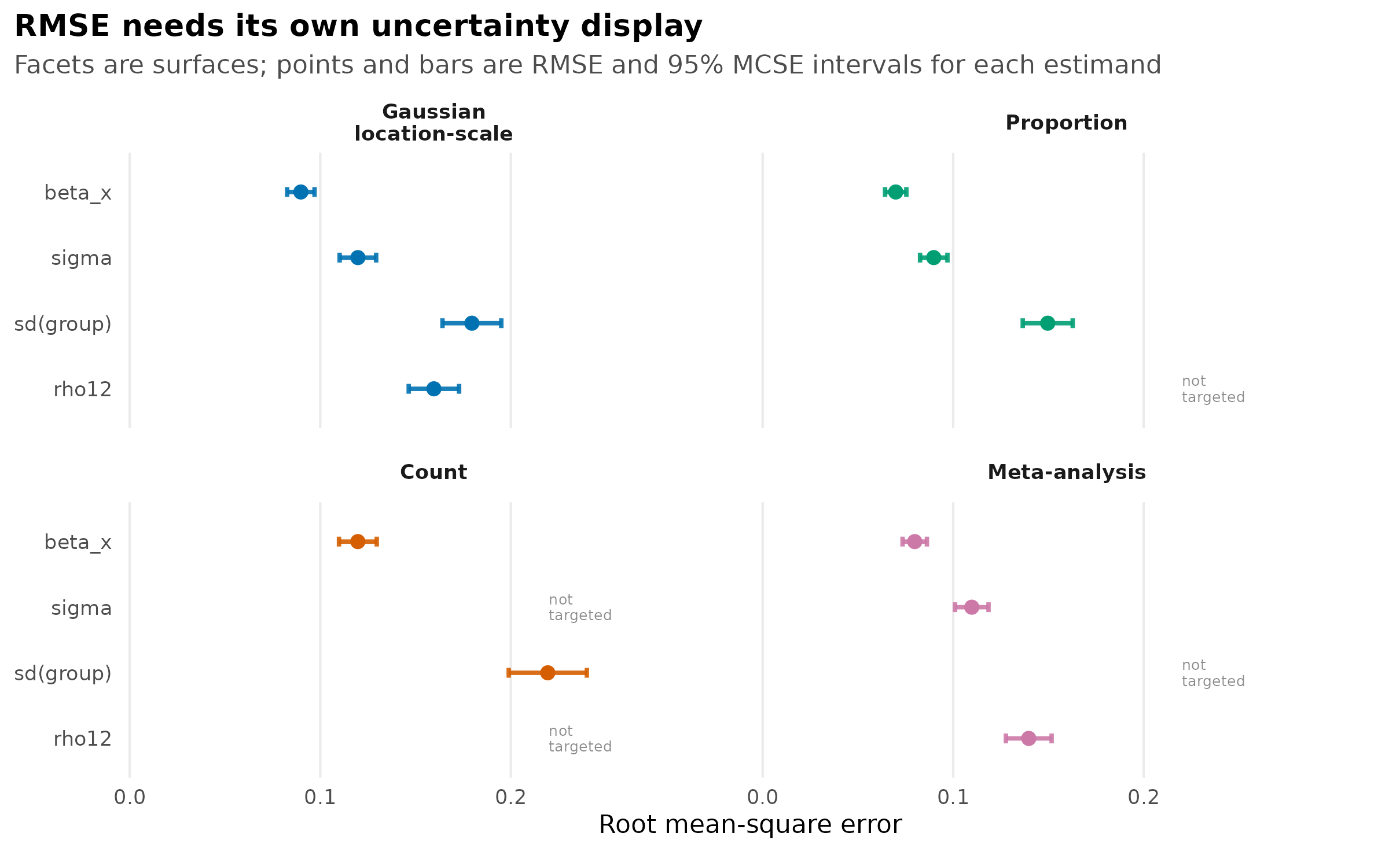
RMSE fixture showing aggregate root-mean-square error points and 95% Monte Carlo standard-error intervals by simulation surface.
The missing rows are part of the message, so unsupported cells stay
visible as not targeted lanes. A count pilot should not
quietly fill rho12 with zeros, and a proportion example
should not invent a random-effect SD if that surface was not fitted.
Real bias reports should replace the fixture quantiles above with one
row per replicate estimate or error, then overplot the aggregate mean
and MCSE interval produced by the Phase 18 summary helpers. RMSE should
remain an aggregate root-mean-square summary with its own MCSE interval,
not a cloud whose center could be mistaken for a mean absolute
error.
Coverage and Power
Coverage and power are proportions, so every point should carry or clearly reference the number of replicates that contributed to it and a Monte Carlo uncertainty interval. Real reports should plot stored replicate rows or stored replicate-block summaries when they are available; the fixture below illustrates that grammar with block-level proportions plus a binomial MCSE approximation for the aggregate.
The example table still carries n_interval for each
cell. The rendered plot keeps the n values out of the panel
labels so the MCSE bars, points, and block-level dots stay aligned and
readable.
interval_summary <- data.frame(
  surface = rep(surface_levels, each = 4),
  estimand = rep(c("beta_x", "sigma", "sd_group", "rho12"), 4),
  coverage = c(
    0.95, 0.93, 0.91, 0.94,
    0.94, 0.92, 0.90, NA,
    0.92, NA, 0.86, NA,
    0.95, 0.94, NA, 0.92
  ),
  power = c(
    0.82, 0.64, 0.58, 0.70,
    0.78, 0.60, 0.52, NA,
    0.74, NA, 0.46, NA,
    0.80, 0.61, NA, 0.66
  ),
  n_interval = c(
    280, 280, 240, 260,
    280, 280, 230, NA,
    250, NA, 200, NA,
    280, 280, NA, 240
  )
)
interval_summary$surface <- factor(
  interval_summary$surface,
  levels = surface_levels
)
interval_long <- rbind(
  data.frame(
    interval_summary[c("surface", "estimand", "n_interval")],
    measure = "Coverage",
    value = interval_summary$coverage,
    target = 0.95
  ),
  data.frame(
    interval_summary[c("surface", "estimand", "n_interval")],
    measure = "Power",
    value = interval_summary$power,
    target = 0.80
  )
)
interval_long$mcse <- sqrt(
  interval_long$value * (1 - interval_long$value) / interval_long$n_interval
)
interval_long$lower <- pmax(0, interval_long$value - 1.96 * interval_long$mcse)
interval_long$upper <- pmin(1, interval_long$value + 1.96 * interval_long$mcse)
interval_long$measure <- factor(
  interval_long$measure,
  levels = c("Coverage", "Power")
)
interval_long$estimand <- factor(
  interval_long$estimand,
  levels = rev(c("beta_x", "sigma", "sd_group", "rho12"))
)
interval_long$missing_x <- ifelse(
  interval_long$measure == "Coverage",
  0.405,
  0.405
)
interval_target <- unique(interval_long[c("measure", "target")])
interval_present <- interval_long[!is.na(interval_long$value), , drop = FALSE]
interval_missing <- interval_long[is.na(interval_long$value), , drop = FALSE]
make_interval_blocks <- function(row, n_block = 18) {
  block_size <- max(8L, floor(row$n_interval / n_block))
  block_proportion <- qbinom(
    ppoints(n_block),
    size = block_size,
    prob = row$value
  ) / block_size
  data.frame(
    surface = row$surface,
    estimand = row$estimand,
    measure = row$measure,
    block_proportion = block_proportion
  )
}
interval_blocks <- do.call(
  rbind,
  lapply(seq_len(nrow(interval_present)), function(i) {
    make_interval_blocks(interval_present[i, ])
  })
)

ggplot(interval_present, aes(value, estimand, colour = surface)) +
  geom_vline(
    data = interval_target,
    aes(xintercept = target),
    linetype = "dotted",
    colour = "grey55",
    inherit.aes = FALSE
  ) +
  geom_point(
    data = interval_blocks,
    aes(block_proportion, estimand, colour = surface),
    position = position_jitter(height = 0.07, width = 0),
    alpha = 0.18,
    size = 0.70,
    inherit.aes = FALSE
  ) +
  geom_segment(
    aes(x = lower, xend = upper, yend = estimand),
    linewidth = 0.4,
    na.rm = TRUE
  ) +
  geom_point(size = 2.1, na.rm = TRUE) +
  geom_text(
    data = interval_missing,
    aes(x = missing_x, y = estimand, label = "not\ntargeted"),
    colour = "grey55",
    size = 2.15,
    lineheight = 0.9,
    hjust = 0,
    inherit.aes = FALSE
  ) +
  facet_grid(
    measure ~ surface,
    labeller = labeller(surface = as_labeller(surface_facet_labels))
  ) +
  scale_colour_manual(values = surface_palette, guide = "none") +
  coord_cartesian(xlim = c(0.38, 1)) +
  scale_x_continuous(
    breaks = c(0.4, 0.6, 0.8, 0.95),
    labels = c("0.40", "0.60", "0.80", "0.95")
  ) +
  scale_y_discrete(labels = estimand_display_labels) +
  labs(
    title = "Interval coverage and power need Monte Carlo uncertainty",
    subtitle = "Faint dots: replicate-block proportions; points/bars: aggregate proportions with 95% binomial MCSE",
    x = "Proportion",
    y = NULL,
    colour = "Surface"
  ) +
  theme_sim_grammar()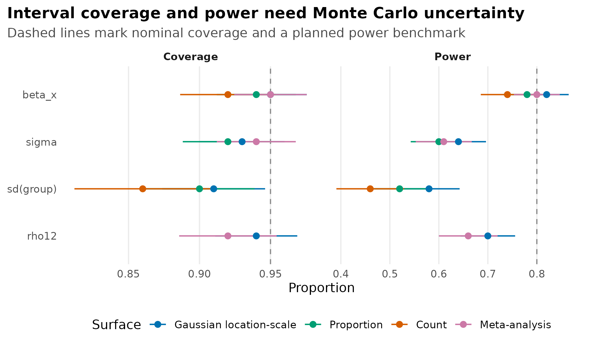
Coverage and power fixture; faint dots are replicate-block proportions, points are aggregate proportions, and horizontal bars are 95% binomial MCSE intervals.
The plot should make pilot status obvious. With few replicates, a coverage estimate near 0.95 can still be too noisy for a release claim.
Convergence and Runtime
Convergence, positive-definite Hessian status, and runtime should sit beside accuracy. A surface with low bias but frequent warnings or high runtime is not ready for broad claims. Fit-status proportions and runtime seconds use separate figures below because they answer related readiness questions on different scales.
ggplot(fit_status_long, aes(value, measure_label, colour = measure)) +
  geom_vline(xintercept = 1, linetype = "dotted", colour = "grey55") +
  geom_segment(
    aes(x = 0, xend = value, yend = measure_label),
    linewidth = 1.2,
    lineend = "round"
  ) +
  geom_point(size = 2.6) +
  facet_wrap(
    ~surface,
    nrow = 1,
    labeller = labeller(surface = as_labeller(surface_facet_labels))
  ) +
  scale_colour_manual(values = c(
    "Converged" = "#0072B2",
    "pdHess" = "#56B4E9"
  )) +
  scale_y_discrete(labels = c(
    "Converged" = "converged",
    "pdHess" = "pdHess"
  )) +
  scale_x_continuous(
    breaks = c(0, 0.5, 1),
    labels = c("0", "0.5", "1"),
    limits = c(0, 1),
    expand = expansion(mult = c(0, 0.03))
  ) +
  labs(
    title = "Fit-status proportions need a readiness row",
    subtitle = "Convergence and pdHess rates stay on a 0-1 scale",
    x = "Fit-status proportion",
    y = NULL,
    colour = "Measure"
  ) +
  guides(colour = "none") +
  theme_sim_grammar() +
  theme(panel.spacing.x = grid::unit(16, "pt"))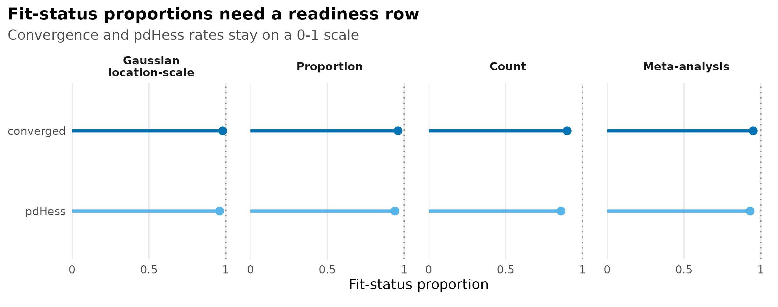
Fit-status readiness fixture showing convergence and positive-definite Hessian proportions on a shared 0-1 scale by simulation surface.
ggplot(runtime_long, aes(value, measure_label, colour = measure)) +
  geom_segment(
    aes(x = 0, xend = value, yend = measure_label),
    linewidth = 1.2,
    lineend = "round"
  ) +
  geom_point(size = 2.6) +
  facet_wrap(
    ~surface,
    nrow = 1,
    labeller = labeller(surface = as_labeller(surface_facet_labels))
  ) +
  scale_colour_manual(values = c(
    "Median runtime" = "#009E73",
    "90th percentile runtime" = "#E69F00"
  )) +
  scale_y_discrete(labels = c(
    "Median runtime" = "median",
    "90th percentile runtime" = "90th pct."
  )) +
  scale_x_continuous(
    breaks = c(0, 0.5, 1, 1.5),
    labels = c("0", "0.5", "1", "1.5"),
    limits = c(0, 1.5),
    expand = expansion(mult = c(0, 0.03))
  ) +
  labs(
    title = "Runtime summaries need a seconds scale",
    subtitle = "Median and 90th percentile rows separate typical from difficult fits",
    x = "Elapsed seconds per fit",
    y = NULL,
    colour = "Measure"
  ) +
  guides(colour = "none") +
  theme_sim_grammar() +
  theme(panel.spacing.x = grid::unit(16, "pt"))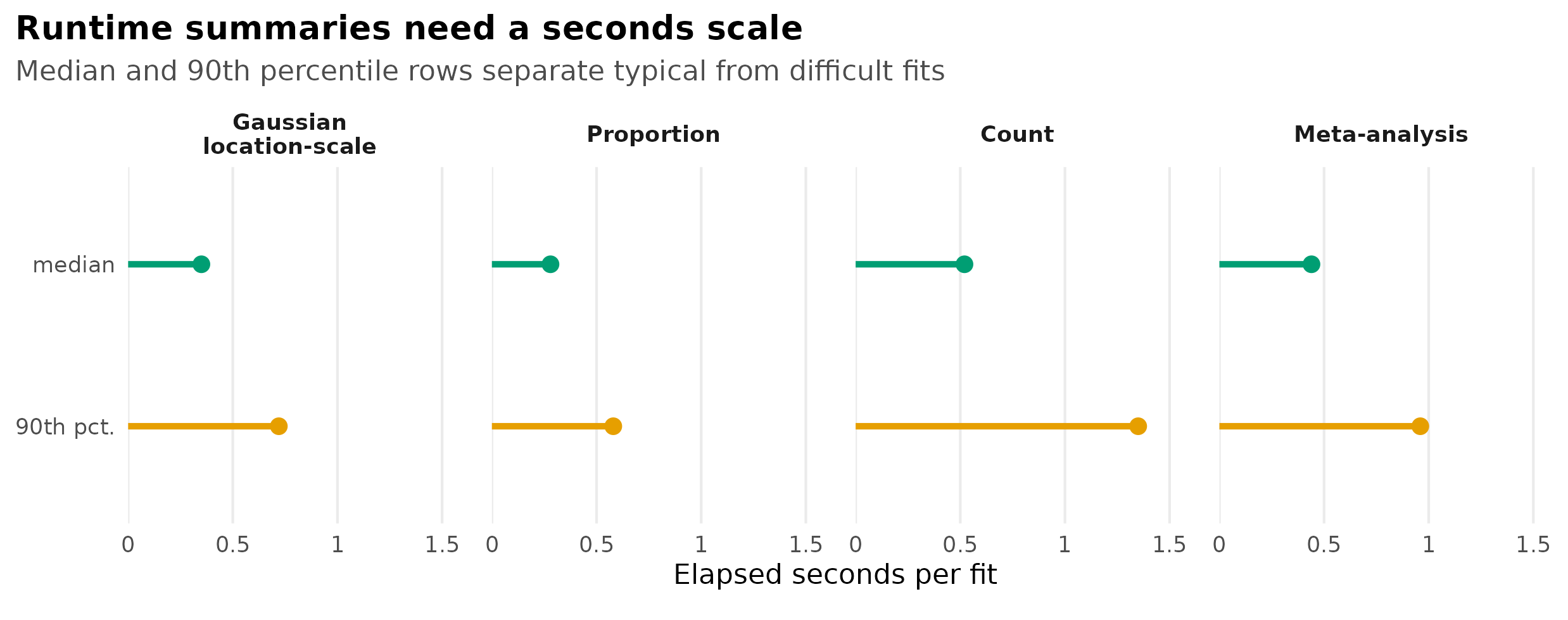
Runtime readiness fixture showing median and 90th percentile elapsed seconds by simulation surface.
Runtime summaries should report medians and high quantiles, not only means, because a few difficult cells can dominate overnight simulation planning.
Failure Ledger
Failures and warnings are data. They should be summarised by surface and condition instead of filtered away before plotting.
failure_ledger <- data.frame(
  surface = rep(surface_levels, each = 5),
  status = rep(c("ok", "warning", "boundary", "error", "skipped"), 4),
  count = c(
    268, 14, 10, 4, 4,
    262, 18, 12, 5, 3,
    232, 30, 20, 12, 6,
    252, 20, 14, 8, 6
  )
)
failure_ledger$surface <- factor(failure_ledger$surface, levels = surface_levels)
failure_ledger$status <- factor(
  failure_ledger$status,
  levels = c("ok", "warning", "boundary", "error", "skipped")
)
failure_ledger$status_label <- factor(
  failure_ledger$status,
  levels = rev(levels(failure_ledger$status))
)

ggplot(failure_ledger, aes(count, status_label, fill = status)) +
  geom_col(width = 0.64) +
  facet_wrap(
    ~surface,
    nrow = 1,
    labeller = labeller(surface = as_labeller(surface_facet_labels))
  ) +
  scale_fill_manual(values = c(
    "ok" = "#009E73",
    "warning" = "#E69F00",
    "boundary" = "#56B4E9",
    "error" = "#D55E00",
    "skipped" = "#999999"
  )) +
  scale_y_discrete(labels = c(
    "ok" = "ok",
    "warning" = "warning",
    "boundary" = "boundary",
    "error" = "error",
    "skipped" = "skipped"
  )) +
  scale_x_continuous(
    breaks = c(0, 25, 100, 200, 300),
    expand = expansion(mult = c(0, 0.04))
  ) +
  labs(
    title = "Warnings and failures stay visible",
    subtitle = "Separate rows keep rare statuses readable beside the dominant ok count",
    x = "Replicate count",
    y = NULL,
    fill = "Status"
  ) +
  guides(fill = "none") +
  theme_sim_grammar()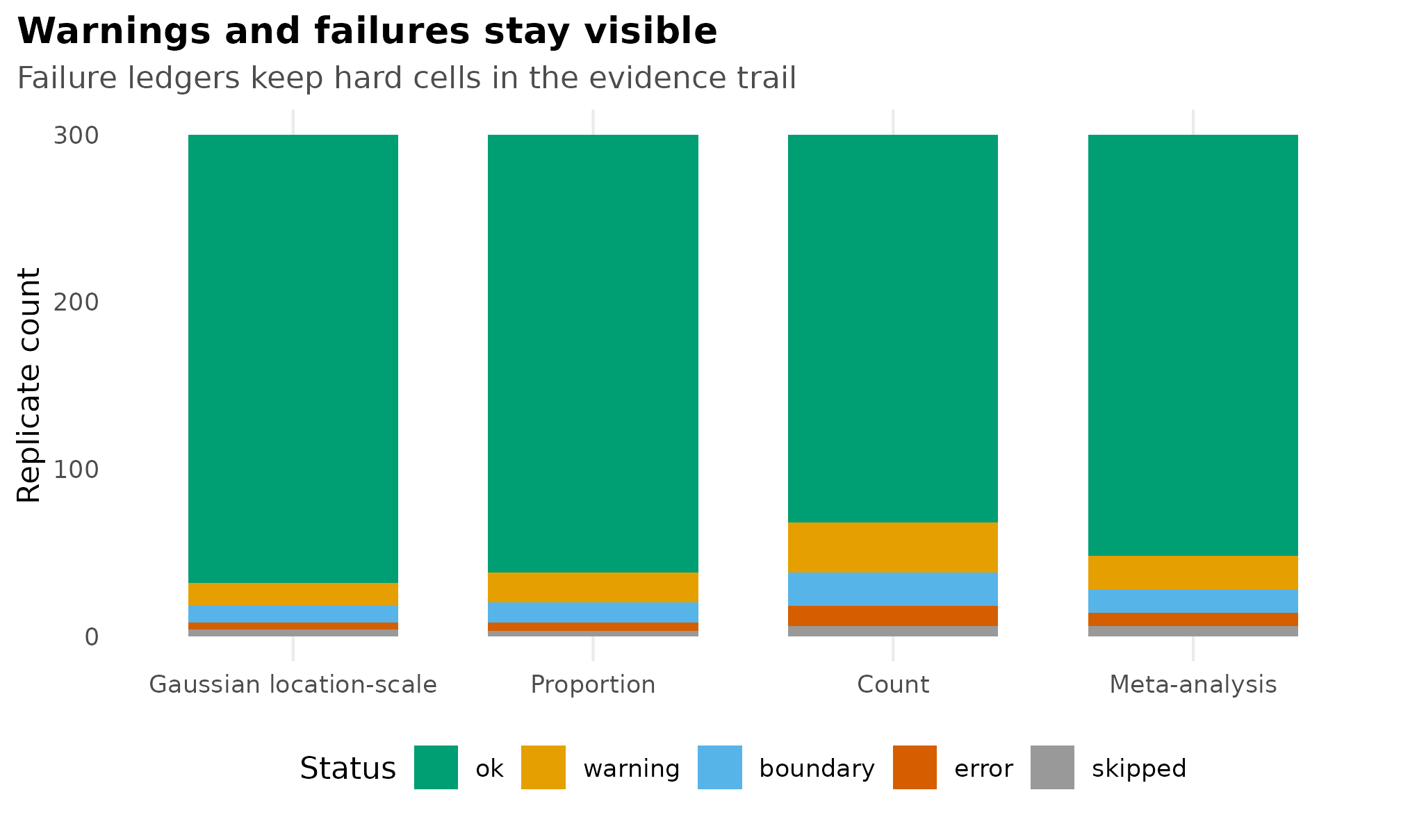
Failure-ledger fixture showing replicate counts by status; warnings, boundary cases, errors, and skipped cells remain visible as separate rows instead of stacked slivers.
Real reports should pair this figure with a table that preserves warning classes, error messages, seeds, and cell identifiers. The plot is for scanning; the ledger is for debugging and reproducibility.
Minimum Table Contract
A real simulation result can add columns, but it should not drop these fields:
| Field | Purpose |
|---|---|
surface |
Human-readable model surface, such as Gaussian location-scale, count, proportion, or meta-analysis |
cell_id |
The varied condition, such as sample size, effect size, true SD, or
known-V structure |
estimand |
The scientific target, such as beta_x,
sigma, sd_group, or rho12
|
truth, estimate, error
|
The value used for bias and RMSE |
conf.low, conf.high,
interval_status
|
The interval source and whether coverage is meaningful |
converged, pdHess,
boundary
|
Fit diagnostics that should be summarised and plotted |
elapsed, warning_count,
error_message
|
Runtime and failure-ledger fields |
n_replicate, mcse
|
Monte Carlo uncertainty for any aggregate claim |
The plotting grammar is deliberately conservative. A feature should not enter a comprehensive plot until the model surface is fitted, the estimand is named, the interval source is known, and failed replicates remain visible.