Working with large data • drmTMB

Large data changes the workflow. A model that is statistically reasonable can still fail because R builds large model frames, dense model matrices, fitted objects, predictions, and residual vectors before the scientific question is answered. This article is for users fitting ecological, evolutionary, or environmental-science models with many observation rows, many species, or both, once the standard post-fit workflow in Checking and using fitted models starts choking on size.

The short version is: fit the smallest model that answers the question, keep only the fitted-object pieces you need, and benchmark on a smaller version of the real data before running the full analysis.

What is implemented now

drmTMB has a first memory-light fitted-object path through drm_control(). For a large univariate Gaussian phylogenetic location model, use:

library(drmTMB)

fit <- drmTMB(
  bf(
    y ~ x1 + x2 + phylo(1 | species, tree = tree),
    sigma ~ 1
  ),
  family = gaussian(),
  data = dat,
  control = drm_control(
    optimizer = list(eval.max = 1000, iter.max = 1000),
    se = FALSE,
    keep_data = FALSE,
    keep_model_frame = FALSE,
    keep_tmb_object = FALSE
  )
)

Here keep_data = FALSE removes the stored complete-case data frame from the fitted object after optimization. keep_model_frame = FALSE removes stored model frames after TMB data are built, including nested model-frame caches for direct random-effect SD models such as sd(species, level = "phylogenetic") ~ z_species and fitted q=2 latent-correlation models such as corpair(...) ~ ecology. se = FALSE skips the TMB::sdreport() step after optimization. The fitted coefficients, fitted values, residuals, prediction, simulation, sigma, rho12, and corpairs() extraction still use the stored model matrices, terms, offsets, response vectors, response-name metadata, random-effect metadata, and optimized parameters. Standard errors, vcov(), and Wald confidence intervals are unavailable in this mode, and summary() marks the standard-error state explicitly. keep_tmb_object = FALSE separately removes the TMB automatic-differentiation object after optimization.

This control is useful when the fitted model is kept for interpretation, prediction, or plotting, but the original data frame and TMB object do not need to travel with it.

For final interval estimates, keep the pieces required by the interval method. Wald intervals need se = TRUE, profile intervals need keep_tmb_object = TRUE, and bootstrap intervals need keep_data = TRUE because the simulated responses are refit with the original model data. Exploratory memory-light fits can therefore use se = FALSE and keep_tmb_object = FALSE, while a final inference refit should keep the standard-error covariance, TMB object, or model data that the chosen interval method needs.

For factor-heavy fixed-effect Gaussian location models, the first sparse fixed-effect path is also available:

fit_sparse <- drmTMB(
  bf(y ~ habitat + x1, sigma ~ 1),
  family = gaussian(),
  data = dat,
  control = drm_control(sparse_fixed = TRUE)
)

This path stores the mu fixed-effect design as a sparse Matrix object and uses a sparse TMB matrix multiply. It is intentionally limited to fixed-effect univariate Gaussian mu models with intercept-only sigma.

For repeated-row Gaussian fixed-effect models, the first aggregation path is also available:

fit_agg <- drmTMB(
  bf(y ~ habitat + season, sigma ~ effort_class),
  family = gaussian(),
  data = dat,
  control = drm_control(aggregate_gaussian = TRUE)
)

This path collapses rows that have the same processed mu and sigma design state after model-row filtering. TMB evaluates the Gaussian likelihood with cell summaries n, sum(y), and sum(y^2), while the fitted object still keeps original-row model matrices and response vectors so predict(fit_agg), fitted(fit_agg), and residuals(fit_agg) return one value per original model row.

What this does not solve yet

The current memory-light path does not prevent R from building model frames and model matrices before optimization. It can drop model frames after fitting, but those objects still need to exist during model construction. That means the control helps fitted-object size, but it is not a complete solution for millions of rows.

These pieces remain planned:

sparse fixed-effect matrices for sigma, random-effect, phylogenetic, spatial, bivariate, and non-Gaussian models;
Gaussian sufficient-statistic aggregation beyond the first fixed-effect univariate path. Random effects, direct-SD formulas, structured effects, known sampling covariance, bivariate Gaussian models, non-Gaussian families, non-unit likelihood weights, and combined sparse fixed-effect matrices are still rejected;
sparse or block-sparse storage for full-matrix meta_V(V = V). The current full known-covariance route keeps the retained V as a dense R matrix and is for small to moderate correlated sampling-error fits;
memory-light modes that avoid constructing dense model frames or dense model matrices in the first place;
repeated benchmark runs for million-row, bivariate, factor-heavy, non-Gaussian, and 10,000-species analyses.

If a model has a high-cardinality factor in a fixed-effect formula, the dense model.matrix() step may dominate memory before TMB sees the data. Treat that as a sparse-design problem, not as a phylogenetic precision problem.

If a model has many repeated Gaussian rows with the same mu and sigma design rows, aggregation is a separate tool from sparse matrices. In the first implemented path, the likelihood uses cell summaries such as n, sum(y), and sum(y^2), but fitted-row summaries remain original-row summaries.

Choose the interval route deliberately

For large phylogenetic Gaussian fits, start with Wald intervals for routine reporting. They are fast and now include direct response-scale targets such as residual sigma and sd:mu:phylo(1 | species) when TMB::sdreport() succeeds:

ci_wald <- confint(
  fit_final,
  parm = c("sigma", "sd:mu:phylo(1 | species)"),
  method = "wald"
)

Use profile intervals when you want a likelihood-based check for a small number of fitted targets. With the default profile_engine = "auto", direct scalar scale, SD, and correlation targets use the endpoint solver instead of building a full adaptive profile curve:

ci_profile <- confint(
  fit_final,
  parm = c("sigma", "sd:mu:phylo(1 | species)"),
  method = "profile"
)

If you need the previous full-profile route for comparison or debugging, ask for it explicitly:

ci_profile_full <- confint(
  fit_final,
  parm = "sd:mu:phylo(1 | species)",
  method = "profile",
  profile_engine = "tmbprofile"
)

On Unix-like systems, parallel = "multicore" can split independent profile targets across workers. For a single direct endpoint target, it can split the lower and upper endpoint searches. When workers = NULL, drmTMB uses about half the detected physical cores, capped at the number of jobs and at 10 workers:

ci_profile_parallel <- confint(
  fit_final,
  parm = c("sigma", "sd:mu:phylo(1 | species)"),
  method = "profile",
  parallel = "multicore",
  workers = NULL
)

Bootstrap intervals are a heavier simulation-refit audit. They require the fitted model data, so do not combine them with drm_control(keep_data = FALSE) unless you refit the final model with keep_data = TRUE first. Use a small R as a smoke test, then increase R only for the final check:

ci_boot <- confint(
  fit_final,
  parm = c("sigma", "sd:mu:phylo(1 | species)"),
  method = "bootstrap",
  R = 99,
  seed = 1,
  parallel = "multicore",
  workers = NULL
)

Treat these routes as different evidence, not as interchangeable defaults. Wald intervals are the routine first pass, endpoint profiles are likelihood-based checks for direct scalar targets, full TMB::tmbprofile() is the debugging and comparison route, and bootstrap is a slower refit-based audit.

The current endpoint benchmark artifact gives a scale for those choices. The plot below uses the synthetic Gaussian phylogenetic benchmark rows recorded in docs/dev-log/benchmarks/profile-scalar-endpoint-v2.csv. It intentionally uses points only: elapsed seconds are local timing measurements from one machine, not confidence intervals.

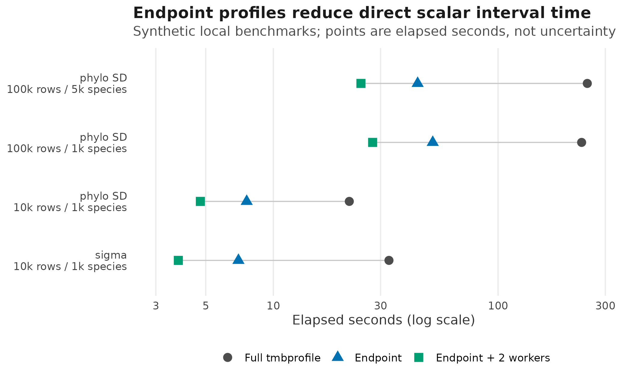
Development benchmark timings for direct scalar profile intervals. Points are elapsed seconds from one local synthetic Gaussian phylogenetic benchmark table; they are performance measurements, not confidence intervals.

Check the fit with the storage choice in mind

Run check_drm() before interpreting a large fit:

check_drm(fit)

If keep_tmb_object = FALSE, the fixed-gradient row is a note rather than an ok result. That note means the gradient cannot be re-evaluated because fit$obj was intentionally dropped. Refit with drm_control(keep_tmb_object = TRUE) when you need the gradient diagnostic for a final report.

If se = FALSE, the sdreport_status, Hessian, and finite-standard-error rows are notes rather than ok results. That note means standard errors were intentionally skipped; refit with drm_control(se = TRUE) when Wald standard errors, vcov(), or Wald confidence intervals are part of the final inference.

The optimizer_budget row compares nlminb() iterations and function evaluations with supplied iter.max and eval.max. If it is a note or warning, inspect convergence, gradients, and model structure before increasing the limits.

Also inspect the fixed_effect_design_size row. It reports the retained fixed-effect design size, the widest design block, the matrix class, and the density of the largest retained block. A dense-fit note with a low density means high-cardinality factors or sparse interactions may be driving memory use before TMB optimization. That is a sparse fixed-effect design problem; simplifying the formula or using drm_control(sparse_fixed = TRUE) when the model is inside the implemented Gaussian mu scope is more relevant than changing the phylogenetic tree.

For full-matrix meta_V(V = V) fits, also inspect the known_sampling_covariance row. It is a note for dense-matrix storage and reports dimension, density, size, rank, and conditioning. A low-density dense V often means the statistical structure is block-sparse, but the current fit has still paid dense R-matrix storage costs.

For aggregated Gaussian fits, check_drm() also includes a gaussian_aggregation row. That row reports the number of original rows, the number of aggregation cells, the compression ratio, and the largest cell size. If the compression ratio is close to 1, aggregation was valid but did not buy much row compression for that model.

Avoid accidental full-row output

Functions such as predict(fit), fitted(fit), residuals(fit), and simulate(fit) can create vectors or data frames with one value per observation. On a five-million-row dataset, that output is itself large.

For interpretation plots, prefer smaller newdata grids:

new_dat <- data.frame(
  x1 = seq(-2, 2, length.out = 100),
  x2 = 0,
  species = dat$species[[1]]
)

predict(fit, newdata = new_dat, dpar = "mu")

For residual checks, decide whether you need every row or a targeted sample. For simulations, start with small nsim and store only the summaries needed for the biological question.

Benchmark before the full run

The repository includes a non-CRAN benchmark harness:

Rscript bench/large-phylo-location.R --rows 100000 --species 1000 \
  --memory-light true --output bench/results.csv

The script generates a synthetic Gaussian phylogenetic location dataset, fits:

y ~ x1 + x2 + phylo(1 | species, tree = tree)
sigma ~ 1

and records elapsed time, fitted-object size, model-matrix size, TMB-data size, the largest retained fixed-effect design block and density, prediction time, residual time, convergence code, optimizer message, optimizer evaluation counts, and fitted scale summaries. Use it to learn how your machine behaves before running the full analysis.

For factor-heavy designs, add:

Rscript bench/large-phylo-location.R --rows 100000 --species 1000 \
  --factor-heavy true --memory-light true --output bench/results.csv

To benchmark the first sparse fixed-effect path, remove the phylogenetic structured effect explicitly:

Rscript bench/large-phylo-location.R --rows 100000 --species 1000 \
  --structured none --factor-heavy true --sparse-fixed true \
  --memory-light true --output bench/results.csv

That sparse smoke scenario fits a fixed-effect Gaussian location model, not a phylogenetic model, because sparse_fixed = TRUE is currently implemented only for univariate Gaussian mu fixed effects with intercept-only sigma.

To benchmark the first Gaussian aggregation path, use a non-phylogenetic repeated-cell scenario:

Rscript bench/large-phylo-location.R --rows 100000 --species 1000 \
  --structured none --aggregate-gaussian true --aggregation-cells 100 \
  --memory-light true --output bench/results.csv

That scenario creates repeated fixed-effect cells deliberately, so the benchmark can record the fitted aggregation-cell count and compression ratio.

For a model with a scale predictor, add:

Rscript bench/large-phylo-location.R --rows 100000 --species 1000 \
  --sigma-x true --memory-light true --output bench/results.csv

The benchmark is intentionally outside the package test suite. It can be slow, and it measures local hardware, BLAS, compiler, and operating-system behaviour as much as package code.

What the current development benchmarks say

The development benchmark table in docs/dev-log/benchmark-results.md records selected local runs. Treat the numbers as planning evidence, not as speed promises for your computer.

Scenario	Local result	What to learn
100k rows, 1k species, ordinary location model	converged; about 25 seconds; about 1.4 GB macOS max RSS	This is the first useful local rung before trying a real large analysis.
100k rows, 5k species	converged; about 32 seconds; about 1.7 GB macOS max RSS	Species-index pressure is separate from row-count pressure.
500k rows, 1k species	converged; about 131 seconds; about 5.1 GB macOS max RSS	Row pressure is feasible on the test machine, but peak memory is already substantial.
100k rows, 1k species, 40-level fixed factor	did not converge under the benchmark optimizer budget	Dense fixed-effect matrices remain a real scaling limitation.

These results support cautious use of the current sparse phylogenetic location path. They do not prove million-row readiness, 10,000-species readiness, bivariate large-data readiness, or non-Gaussian large-data readiness.

Practical checklist

Start with a fixed-effect or smaller phylogenetic model that answers a simpler version of the question.
Fit with keep_data = FALSE, keep_model_frame = FALSE, se = FALSE, and keep_tmb_object = FALSE when you do not need to carry the original data, model frames, standard-error covariance, or TMB object inside the saved fit.
Refit the final model with se = TRUE for Wald intervals, keep_tmb_object = TRUE for profile intervals, and keep_data = TRUE for bootstrap intervals.
Use Wald intervals first for direct sigma, structured SD, and correlation targets; use endpoint profile intervals as a likelihood-based check on the few targets that matter most.
Keep keep_tmb_object = TRUE for final diagnostic refits where the fixed gradient check matters.
Inspect check_drm(fit) for fixed-effect design-size notes before assuming the phylogenetic part caused memory pressure.
Use newdata grids for interpretation instead of creating full-row predictions by default.
Run the benchmark script at 100k rows before trying million-row analyses.
Treat a non-zero optimizer code as a diagnostic result, not as timing evidence.
Treat sparse fixed-effect matrices outside fixed-effect Gaussian mu models, and data aggregation in all models, as future scaling features rather than current guarantees.