Coordinate-spatial structured effects

Use spatial() when named sites have coordinates and nearby sites may have similar location deviations after fixed effects have been included. The fitted route uses a coordinate table supplied as coords = coords. Mesh and SPDE inputs remain planned. If distance between sites is not what couples your observations, the structural-dependence overview compares this route against the relatedness- and tree-based ones.

What is fitted today

Question	Syntax	Status
Does one Gaussian response have smooth site-level location deviations?	spatial(1 | site, coords = coords) in mu	Fitted first coordinate-spatial intercept slice.
Does one predictor have a spatially varying slope?	spatial(1 + depth | site, coords = coords) in mu	Fitted one numeric-slope slice. The intercept and slope fields are independent and have separate SDs.
Do two Gaussian response means share a coordinate-spatial correlation?	matching spatial(1 | p | site, coords = coords) terms in mu1 and mu2	Fitted q=2 location-location slice. corpairs(level = "spatial") reports the latent spatial row separately from residual rho12.
Do spatial location and scale deviations covary across two Gaussian responses?	matching spatial(1 | p | site, coords = coords) terms in mu1, mu2, sigma1, and sigma2	Fitted constant q=4 location-scale slice. Six latent spatial rows are reported through corpairs(level = "spatial"); q=4 correlations are derived and unavailable for intervals.

Start with the smallest useful model

For one response, start with a coordinate-spatial location intercept:

fit_spatial <- drmTMB(
  y ~ treatment + spatial(1 | site, coords = coords),
  data = dat,
  family = gaussian()
)

Add one numeric slope only when the scientific question is about spatial variation in that slope:

fit_spatial_slope <- drmTMB(
  y ~ treatment + depth + spatial(1 + depth | site, coords = coords),
  data = dat,
  family = gaussian()
)

For the exact Arc 1a REML route, keep sigma ~ 1, use an unlabelled intercept or independent intercept-plus-one-numeric-slope shape, and set REML = TRUE:

fit_spatial_reml <- drmTMB(
  bf(
    y ~ depth + spatial(1 + depth | site, coords = coords),
    sigma ~ 1
  ),
  data = dat,
  family = gaussian(),
  REML = TRUE
)

The multi-seed campaign used the coordinate representation shown here, with n_each = 20 and exactly M = {8, 16, 32} sites. This is not a continuous minimum-sample-size claim, and it does not admit estimated range, labelled, slope-only, multiple-slope, scale-side, other bivariate, or non-Gaussian REML routes. The exact bivariate exception is the matched labelled location-intercept cell below.

For two response means, use matching labelled terms and read the latent spatial correlation with corpairs():

fit_spatial_q2 <- drmTMB(
  mu1 = trait1 ~ treatment +
    spatial(1 | p | site, coords = coords),
  mu2 = trait2 ~ treatment +
    spatial(1 | p | site, coords = coords),
  data = dat,
  family = biv_gaussian()
)
corpairs(fit_spatial_q2, level = "spatial")
rho12(fit_spatial_q2)

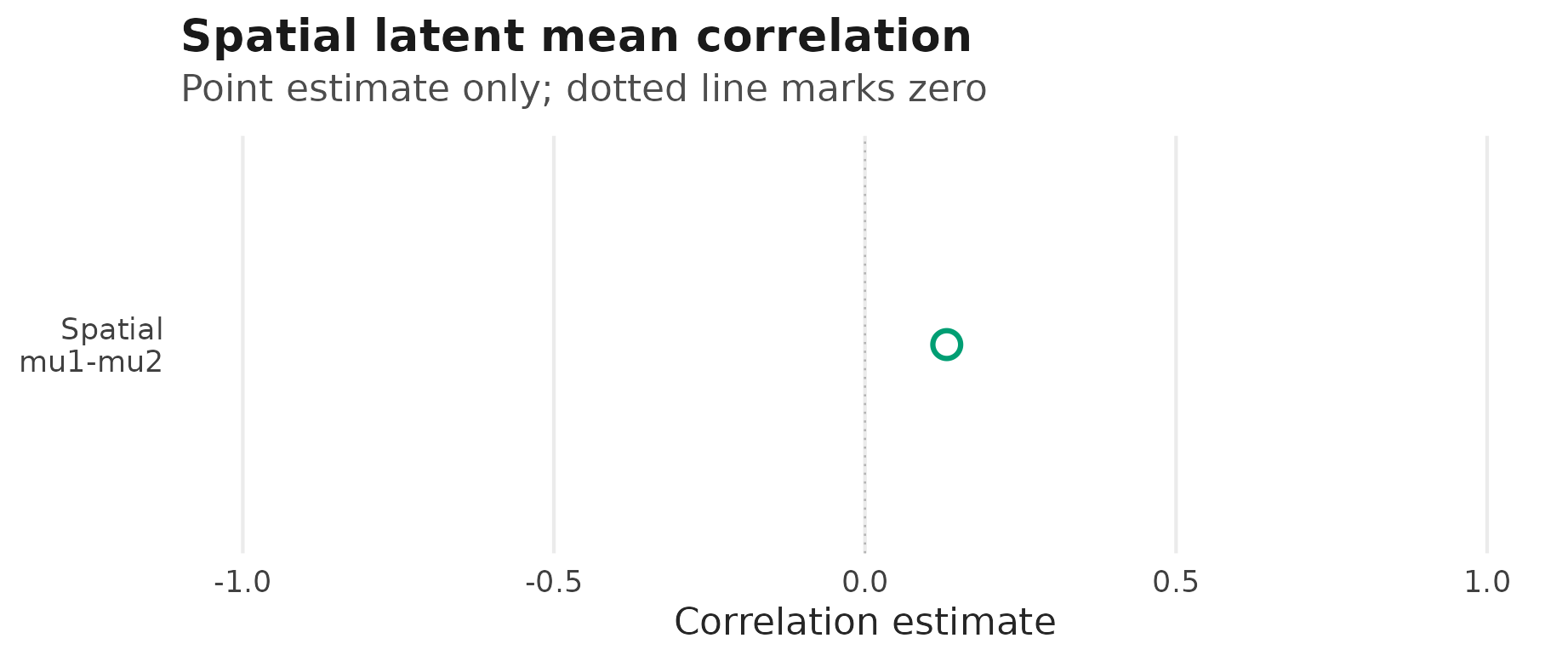
corpairs() reports the fitted latent coordinate-spatial correlation among site-level location deviations. rho12() reports the residual correlation between paired responses after fixed effects and random effects have been included.

That exact q2 location-intercept model also admits native REML when the three residual parameters are intercept-only:

fit_spatial_q2_reml <- drmTMB(
  bf(
    mu1 = trait1 ~ treatment +
      spatial(1 | p | site, coords = coords),
    mu2 = trait2 ~ treatment +
      spatial(1 | p | site, coords = coords),
    sigma1 = ~ 1,
    sigma2 = ~ 1,
    rho12 = ~ 1
  ),
  data = dat,
  family = biv_gaussian(),
  REML = TRUE
)

Here the coordinates define a fixed spatial covariance matrix. This cell has dense-oracle and retained-denominator point-recovery evidence only; it does not authorize interval, coverage, range-estimation, slope, scale-side, or q4 claims.

For a constant location-scale spatial block, use the same labelled spatial() term in all four bivariate Gaussian endpoints:

fit_spatial_q4 <- drmTMB(
  mu1 = trait1 ~ treatment +
    spatial(1 | p | site, coords = coords),
  mu2 = trait2 ~ treatment +
    spatial(1 | p | site, coords = coords),
  sigma1 = ~ treatment +
    spatial(1 | p | site, coords = coords),
  sigma2 = ~ treatment +
    spatial(1 | p | site, coords = coords),
  rho12 = ~ 1,
  data = dat,
  family = biv_gaussian()
)
corpairs(fit_spatial_q4, level = "spatial")

This q=4 route estimates four coordinate-spatial endpoint SDs and six latent correlations: one location-location, four location-scale, and one scale-scale row. It is still a constant intercept block, not a spatial slope or predictor-dependent spatial correlation model.

What to inspect

After fitting, inspect the spatial layer before interpreting it:

Output	Use
check_drm(fit)	Confirm the spatial layer was recognized and review coordinate/site diagnostics.
fit$sdpars$mu	Read fitted spatial location SDs, including separate intercept and slope SDs when a one-slope model is used.
ranef(fit, "spatial_mu")	Inspect conditional site deviations on the fitted spatial layer.
summary(fit)$covariance	Check how spatial SDs and q=2 or q=4 spatial correlations are reported beside other covariance layers.
profile_targets(fit)	See which spatial SD or constant q=2 correlation targets can be profiled directly, and which q=4 correlation rows are derived-unavailable for intervals.
corpairs(fit, level = "spatial")	Read fitted constant spatial correlation rows.

The one-slope route is deliberately narrow. The formula term spatial(1 + depth | site, coords = coords) fits an intercept field and one numeric slope field with the same coordinate precision and separate SDs. It does not estimate an intercept-slope correlation. Spatial sigma is supported through a separate route – a standalone sigma ~ spatial(1 | site) or sigma ~ spatial(1 + depth | site) field, or the matched location-scale block – which fits at recovery grade (trust the point estimate, not the interval); this mu one-slope term is not that route.

Rendered checks

The small example below is only a guide to the output grain. The coordinate surface is fitted in the location predictor mu; raw response values remain on the response scale and should not be plotted as if they were spatial SDs or correlations.

spatial_example <- simulate_spatial_guide_data()
spatial_dat <- spatial_example$data
coords <- spatial_example$coords

fit_spatial <- drmTMB(
  drm_formula(
    y ~ depth + temp + spatial(1 | site, coords = coords),
    sigma ~ depth
  ),
  family = gaussian(),
  data = spatial_dat
)

fit_spatial_slope <- drmTMB(
  drm_formula(
    y ~ depth + temp + spatial(1 + depth | site, coords = coords),
    sigma ~ depth
  ),
  family = gaussian(),
  data = spatial_dat
)

if (requireNamespace("ggplot2", quietly = TRUE)) {
  spatial_effect <- ranef(fit_spatial, "spatial_mu")$terms[[1]]
  spatial_field <- data.frame(
    site = names(spatial_effect),
    fitted_spatial_deviation = unname(spatial_effect),
    coords[names(spatial_effect), , drop = FALSE],
    row.names = NULL
  )

  ggplot2::ggplot(
    spatial_field,
    ggplot2::aes(
      x = x,
      y = y,
      fill = fitted_spatial_deviation
    )
  ) +
    ggplot2::geom_hline(yintercept = 0, colour = "grey90", linewidth = 0.4) +
    ggplot2::geom_vline(xintercept = 0, colour = "grey90", linewidth = 0.4) +
    ggplot2::geom_point(
      shape = 21,
      size = 7,
      colour = "grey20",
      linewidth = 0.35
    ) +
    ggplot2::scale_fill_gradient2(
      low = "#D55E00",
      mid = "white",
      high = "#009E73",
      midpoint = 0,
      name = "Fitted\nspatial deviation"
    ) +
    ggplot2::coord_equal() +
    spatial_guide_theme() +
    ggplot2::labs(
      title = "Fitted spatial location field",
      subtitle = "Conditional deviations in mu",
      x = "Coordinate x",
      y = "Coordinate y"
    )
}
#> Warning in ggplot2::geom_point(shape = 21, size = 7, colour = "grey20", :
#> Ignoring unknown parameters: `linewidth`

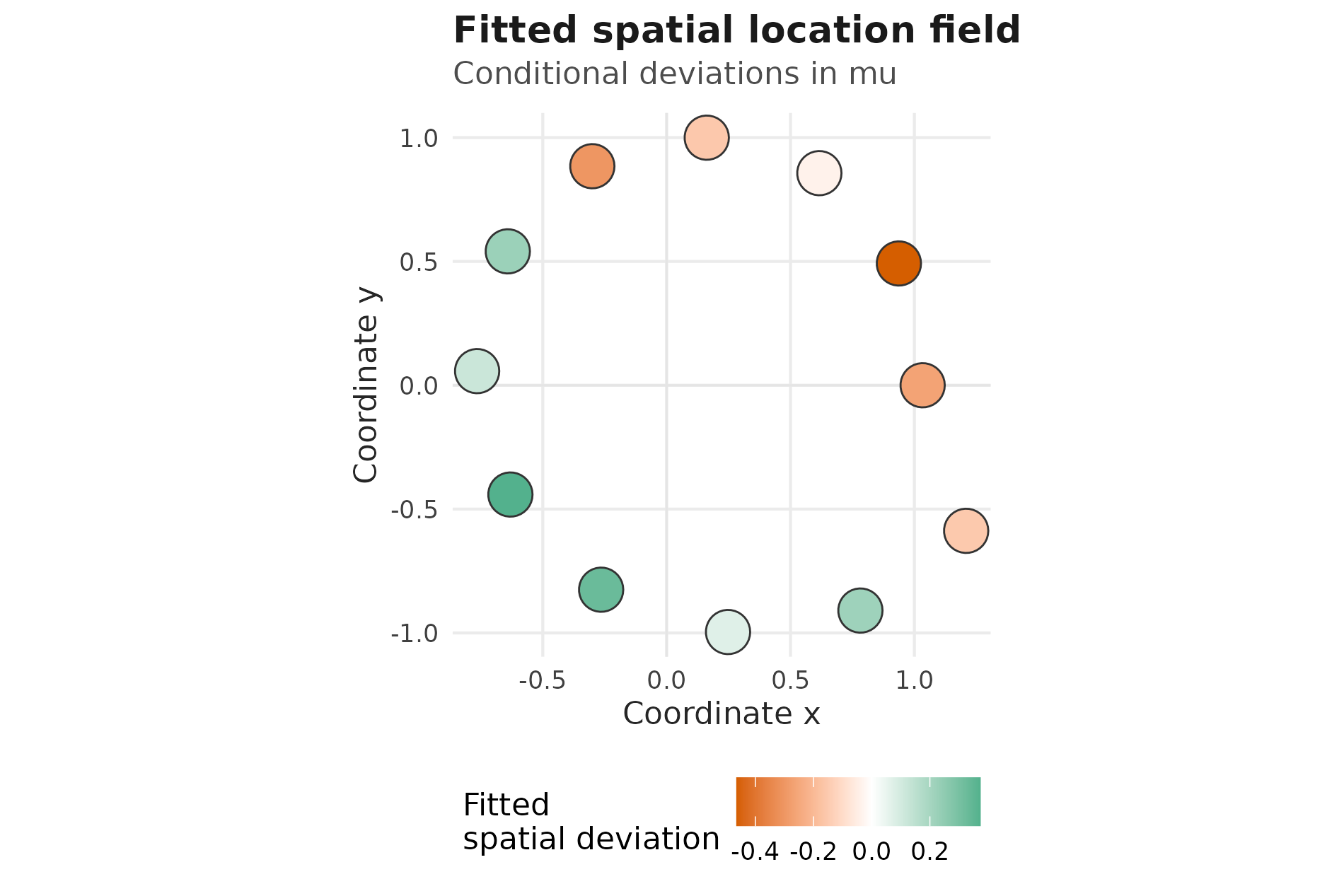
Coordinate-spatial fitted site deviations from ranef(fit_spatial, "spatial_mu"); points are conditional location-effect estimates, and no interval is drawn because this display is a site-level fitted field rather than a confidence-interval summary.

if (requireNamespace("ggplot2", quietly = TRUE)) {
  spatial_sd <- data.frame(
    estimate = unname(fit_spatial_slope$sdpars$mu[
      c("spatial(1 | site)", "spatial(0 + depth | site)")
    ]),
    label = c("Spatial\nintercept SD", "Spatial\ndepth-slope SD"),
    unit = c("Response units", "Response units per depth unit")
  )

  ggplot2::ggplot(spatial_sd, ggplot2::aes(y = label)) +
    ggplot2::geom_vline(
      xintercept = 0,
      linewidth = 0.45,
      linetype = "dashed",
      colour = "grey55"
    ) +
    ggplot2::geom_point(
      ggplot2::aes(x = estimate),
      shape = 21,
      size = 3.5,
      stroke = 1,
      fill = "white",
      colour = "#0072B2"
    ) +
    ggplot2::scale_x_continuous(
      expand = ggplot2::expansion(mult = c(0.01, 0.04))
    ) +
    spatial_eye_theme() +
    ggplot2::labs(
      title = "Spatial intercept and slope SDs have different units",
      subtitle = "Point estimates only; interval validation remains planned",
      x = "Fitted spatial standard deviation",
      y = NULL
    )
}

Fitted coordinate-spatial intercept-field SD (response units) and depth-slope field SD (response units per unit depth) from the one-slope model. Interval calibration for these exact rows is not validated, so no interval bars are drawn.

For bivariate spatial location models, the current intercept-only q2 corpairs() row is point-only: profile mechanics exist, but interval calibration and coverage remain planned. Native REML for this exact cell requires complete response pairs, unit weights, intercept-only sigma1, sigma2, and rho12, no known meta_V() covariance, and no additional ordinary random effect, direct-SD formula, or corpair() regression. The raw paired responses do not belong on this axis.

spatial_q2_example <- simulate_spatial_q2_guide_data()
spatial_q2_dat <- spatial_q2_example$data
spatial_q2_coords <- spatial_q2_example$coords

fit_spatial_q2_example <- drmTMB(
  drm_formula(
    mu1 = y1 ~ x + spatial(1 | p | site, coords = spatial_q2_coords),
    mu2 = y2 ~ x + spatial(1 | p | site, coords = spatial_q2_coords),
    sigma1 = ~ 1,
    sigma2 = ~ 1,
    rho12 = ~ 1
  ),
  family = c(gaussian(), gaussian()),
  data = spatial_q2_dat
)

spatial_q2_pairs <- suppressWarnings(
  corpairs(
    fit_spatial_q2_example,
    level = "spatial"
  )
)
spatial_q2_pairs
#>     level group block from_dpar to_dpar   from_coef     to_coef from_response
#> 1 spatial  site     p       mu1     mu2 (Intercept) (Intercept)            y1
#>   to_response     class                                       parameter
#> 1          y2 mean-mean cor(mu1:(Intercept),mu2:(Intercept) | p | site)
#>    estimate       min       max n_values link_estimate  link_min  link_max
#> 1 0.1314222 0.1314222 0.1314222        1     0.1321869 0.1321869 0.1321869
#>   modelled   conf.status interval_source
#> 1    FALSE not_requested   not_available

if (requireNamespace("ggplot2", quietly = TRUE)) {
  spatial_q2_display <- spatial_q2_pairs
  spatial_q2_display$display_label <- "Spatial\nmu1-mu2"

  plot_corpairs(
    spatial_q2_display,
    colour = "level",
    label = "display_label",
    facet = NULL
  ) +
    ggplot2::scale_colour_manual(values = c("spatial" = "#009E73")) +
    ggplot2::scale_fill_manual(values = c("spatial" = "#009E73")) +
    spatial_eye_theme() +
    ggplot2::labs(
      title = "Spatial latent mean correlation",
      subtitle = "Point estimate only; dotted line marks zero",
      x = "Correlation estimate"
    )
}
#> Warning: No shared levels found between `names(values)` of the manual scale and the
#> data's fill values.

Coordinate-spatial intercept-only q=2 location-location point estimate from corpairs(); the dotted vertical line marks zero correlation and no interval is shown because calibration remains planned.

Boundaries

The following spatial routes remain planned:

• mesh or SPDE inputs such as spatial(1 | site, mesh = mesh);
• multiple spatial slopes and spatial slope correlations;
• partial spatial terms in sigma, plus spatial terms in nu, zero-inflation, or rho12;
• direct spatial SD surfaces;
• predictor-dependent spatial corpair() regressions;
• simultaneous phylo() plus spatial() layers in the same formula;
• non-Gaussian spatial structured effects outside the exact ordinary Poisson/NB2 q1 spatial mu intercept-plus-one-slope, recovery-grade NB2 q1 spatial sigma, Student-t spatial mu, Poisson spatial zi, fixed-zi Poisson spatial mu, and fixed-zi NB2 spatial mu gates.

Use the structural-dependence overview when you are choosing among animal(), phylo(), spatial(), and relmat(). Use the detailed structural-dependence tutorial when you need the current worked examples, equations, and broader parity ladder. ggplot2::facet_grid(unit ~ ., scales = “free_x”, space = “free_y”) + ggplot2::theme(strip.text.y = ggplot2::element_text(angle = 0)) +