Animal models and additive relatedness • drmTMB

Use animal() when individuals have known additive relatedness and the scientific question is about among-individual location deviations after the fixed effects have been included. The fitted first slices are Gaussian location models. They are useful for animal-model and quantitative-genetic workflows, but they are not yet full parity with every phylo() route. This page assumes a pedigree or additive-relatedness matrix is already the right description of your data; the structural-dependence overview is where that choice gets made.

What is fitted today

Question	Syntax	Status
Does one Gaussian response have additive individual deviations?	`animal(1 \| individual, pedigree = pedigree)`, `animal(1 \| individual, A = A)`, or `animal(1 \| individual, Ainv = Ainv)` in `mu`	Fitted first slice. Dense pedigree construction, covariance input, and precision input are supported.
Does one numeric fixed-effect slope also have additive individual deviations?	`animal(1 + x \| individual, pedigree = pedigree)` in `mu`	Fitted first univariate one-slope slice with independent intercept and slope fields. Additional structured-slope layouts outside the exact fitted bivariate ledger cells and intercept-slope correlations remain planned.
Does a one-response Gaussian model have additive residual-scale deviations?	`animal(1 \| individual, Ainv = Ainv)` in `sigma`, alone or matching the `mu` term; `animal(1 + x \| individual, A = A)` for the exact one-slope route	The residual-scale intercept is fitted. The exact A-matrix q1 `sigma` one-slope route is fitted and inference-ready with caveats under raw uncorrected log-SD Wald-z intervals; profile is diagnostic-only at `g = 8`. Matching univariate `mu` and `sigma` animal intercepts estimate one animal mean-scale correlation. Pedigree/Ainv bridge marshalling, additional multiple or labelled sigma-slope layouts outside the exact fitted bivariate ledger cells, and structured slope correlations remain planned.
Do two Gaussian response means share an animal-model correlation?	matching labelled `animal(1 \| p \| individual, pedigree = pedigree)`, `animal(1 \| p \| individual, A = A)`, or `animal(1 \| p \| individual, Ainv = Ainv)` terms in `mu1` and `mu2`	Fitted first q=2 location-location slice. `corpairs(level = "animal")` reports the latent animal correlation separately from residual `rho12`.
Do animal-model deviations link means and residual scales across two responses?	the same labelled `animal(1 \| p \| individual, Ainv = Ainv)` term in `mu1`, `mu2`, `sigma1`, and `sigma2`	Fitted first q=4 location-scale slice. `corpairs(level = "animal")` reports six constant latent animal correlations; profile intervals for those derived correlations remain unavailable.
Does the animal effect change multiple slopes or a predictor-dependent correlation?	examples such as `animal(1 + x + z \| individual, pedigree = pedigree)` or animal `corpair()` formulas	Planned. These routes need separate diagnostics, recovery tests, interval targets, and examples before use.

The pedigree route expects a data frame whose identifiers match the grouping variable used in the formula. The A route uses a precomputed additive relationship covariance matrix, and the Ainv route uses the corresponding precision matrix. Use exactly one of pedigree, A, or Ainv for a fitted animal term.

Start with the smallest useful model

For one response, start with the fitted location-intercept route:

fit_animal <- drmTMB(
  y ~ treatment + animal(1 | individual, pedigree = pedigree),
  data = dat,
  family = gaussian()
)

For the exact Arc 1a REML route, keep sigma ~ 1, use an unlabelled intercept or independent intercept-plus-one-numeric-slope shape, and set REML = TRUE:

fit_animal_reml <- drmTMB(
  bf(
    y ~ x + animal(1 + x | individual, A = A),
    sigma ~ 1
  ),
  data = dat,
  family = gaussian(),
  REML = TRUE
)

The multi-seed campaign used the A representation shown here, with n_each = 20 and one fixed M = 8 relationship matrix. Pedigree and Ainv inputs have deterministic representation-parity evidence only, not multi-seed campaign coverage. These domains do not admit slope-only, labelled, multiple-slope, scale-side, bivariate, or non-Gaussian REML routes.

For two responses, use the same animal block label in mu1 and mu2:

fit_animal_q2 <- drmTMB(
  bf(
    mu1 = trait1 ~ treatment +
      animal(1 | p | individual, Ainv = Ainv),
    mu2 = trait2 ~ treatment +
      animal(1 | p | individual, Ainv = Ainv)
  ),
  data = dat,
  family = biv_gaussian()
)
corpairs(fit_animal_q2, level = "animal")
rho12(fit_animal_q2)

The two extractors answer different questions. corpairs() reports the fitted latent animal-model correlation among individual location deviations. rho12() reports the residual correlation between the two responses after the fixed effects and random effects have been included.

For reports, keep this intercept-only q=2 animal correlation point-only. The profile mechanism computes, but interval calibration and coverage are still planned for this row:

animal_pairs <- corpairs(fit_animal_q2, level = "animal")
plot_corpairs(animal_pairs)

That plot should be read as an animal-layer correlation display, not as a residual rho12 plot. Do not add an interval eye until this exact row has validated interval evidence. The q=4 rows below are also point-only: current q=4 animal correlations are derived rows.

When the biological question is whether additive individual deviations in means and residual scales covary, use the same labelled animal term in all four bivariate endpoint formulas:

fit_animal_q4 <- drmTMB(
  bf(
    mu1 = trait1 ~ treatment +
      animal(1 | p | individual, Ainv = Ainv),
    mu2 = trait2 ~ treatment +
      animal(1 | p | individual, Ainv = Ainv),
    sigma1 = ~ treatment +
      animal(1 | p | individual, Ainv = Ainv),
    sigma2 = ~ treatment +
      animal(1 | p | individual, Ainv = Ainv)
  ),
  data = dat,
  family = biv_gaussian()
)
corpairs(fit_animal_q4, level = "animal")

The q=4 path is constant across individuals and responses: it estimates four latent animal endpoint scale parameters and six latent animal correlations. Each endpoint’s individual marginal SD also includes sqrt(A[i, i]). This is not a direct-SD model and it does not make the residual correlation rho12 animal-structured.

What to inspect

After fitting, inspect the animal layer before interpreting it:

Output	Use
`check_drm(fit)`	Confirm the structured layer was recognized and review convergence diagnostics.
`fit$sdpars$mu`	Read the fitted latent animal scale `s`; individual `i` has marginal SD `s sqrt(A[i, i])`.
`ranef(fit, "animal_mu")`	Inspect conditional individual deviations on the fitted animal layer.
`summary(fit)$covariance`	Check how the animal SD or correlation is reported beside other covariance layers.
`profile_targets(fit)`	See which animal SD or q=2 correlation targets can be profiled directly; q=4 correlations are derived-only in the first slice.
`corpairs(fit, level = "animal")`	Read the fitted q=2 animal mean-mean correlation, or the six q=4 animal endpoint correlations when the model has the all-four block.

If the ordinary repeatability model answers a useful sensitivity question, fit (1 | individual) as a comparison. Report it as an ordinary individual random-effect model, not as an additive animal model.

Rendered checks

The small examples below keep three evidence grains separate. The relationship matrix is raw structure supplied to the model. The SD plot converts the fitted latent scale s to individual marginal SDs s sqrt(A[i, i]) before comparing them with residual sigma; it omits uncertainty intervals because the animal q1 location-SD row is not interval-validated. The q=2 animal-correlation plot is also a fitted point estimate from corpairs() with a dotted zero line; its interval calibration remains planned.

animal_example <- simulate_animal_guide_data()
animal_dat <- animal_example$data
A <- animal_example$A
Ainv <- animal_example$Ainv

fit_animal <- drmTMB(
  bf(
    body_size ~ age + sex + animal(1 | individual, Ainv = Ainv),
    sigma ~ 1
  ),
  family = gaussian(),
  data = animal_dat
)

if (requireNamespace("ggplot2", quietly = TRUE)) {
  animal_matrix <- relatedness_heatmap_data(A)

  ggplot2::ggplot(
    animal_matrix,
    ggplot2::aes(column, row, fill = relatedness)
  ) +
    ggplot2::geom_tile() +
    ggplot2::coord_equal() +
    ggplot2::scale_fill_gradientn(
      colours = c("#F7FBFF", "#C6DBEF", "#6BAED6", "#08519C"),
      name = "Additive\nrelatedness"
    ) +
    animal_guide_theme() +
    ggplot2::theme(
      axis.text = ggplot2::element_blank(),
      axis.ticks = ggplot2::element_blank(),
      panel.grid = ggplot2::element_blank()
    ) +
    ggplot2::labs(
      title = "Animal-model input structure",
      subtitle = "Known additive relatedness among individuals",
      x = "Individual",
      y = "Individual"
    )
}

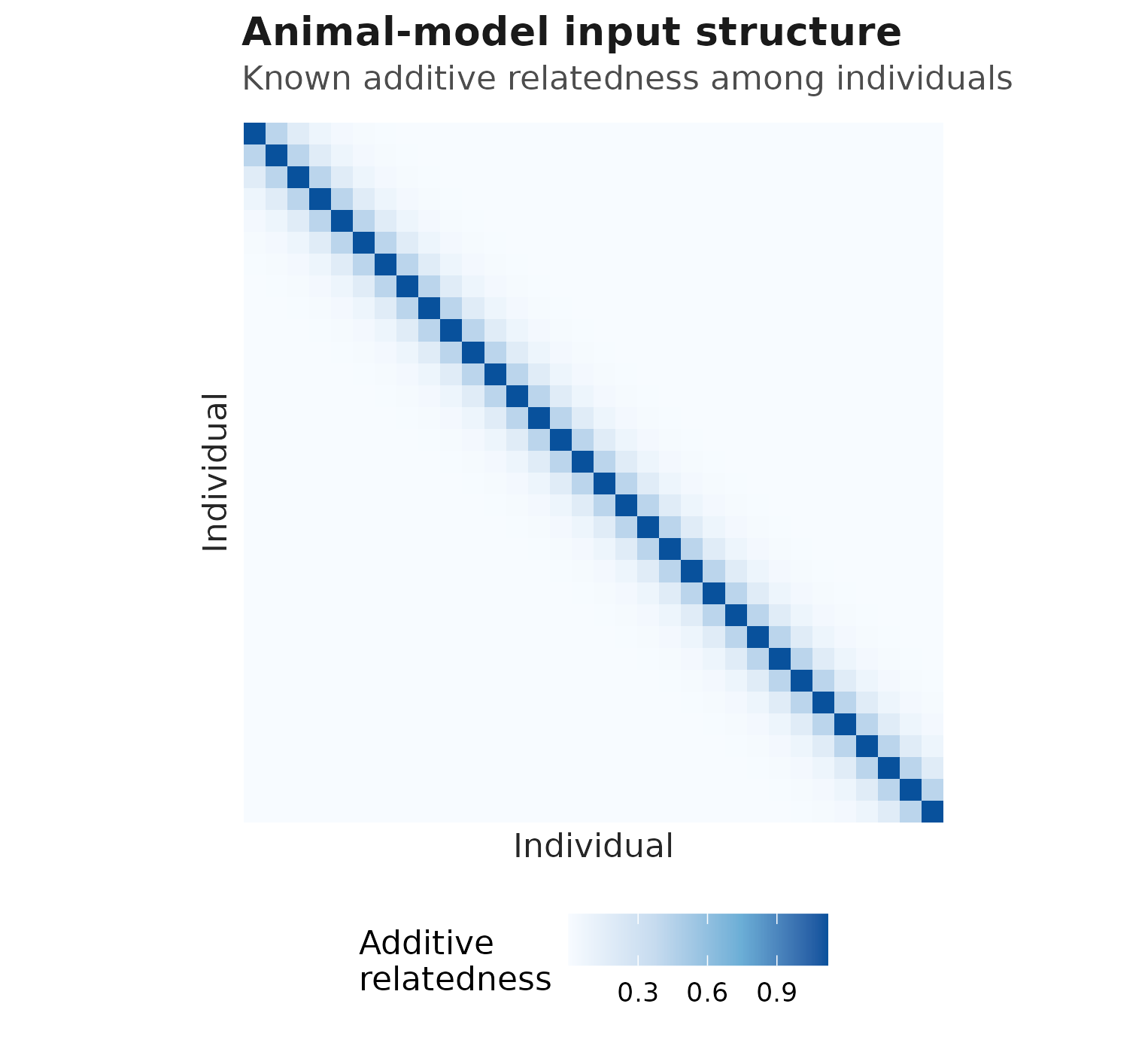
Heatmap of the additive relatedness matrix for the animal-model example. Values are highest on the diagonal and fade as individuals are farther apart in the simulated pedigree-like ordering.

Additive relatedness matrix used by the animal-model example; this heatmap is the known input structure, not an uncertainty display.

if (requireNamespace("ggplot2", quietly = TRUE)) {
  animal_scale <- unname(fit_animal$sdpars$mu["animal(1 | individual)"])
  animal_node_sd <- animal_scale * sqrt(diag(A))
  animal_sd <- data.frame(
    estimate = c(
      unname(exp(coef(fit_animal, "sigma")["(Intercept)"])),
      animal_node_sd
    ),
    label = c(
      "Residual\nsigma",
      rep("Animal node\nmarginal SD", length(animal_node_sd))
    )
  )

  ggplot2::ggplot(animal_sd, ggplot2::aes(y = label)) +
    ggplot2::geom_vline(
      xintercept = 0,
      linewidth = 0.45,
      linetype = "dashed",
      colour = "grey55"
    ) +
    ggplot2::geom_point(
      ggplot2::aes(x = estimate),
      shape = 21,
      size = 3.5,
      stroke = 1,
      fill = "white",
      colour = "#0072B2"
    ) +
    ggplot2::scale_x_continuous(
      expand = ggplot2::expansion(mult = c(0.02, 0.05))
    ) +
    animal_eye_theme() +
    ggplot2::labs(
      title = "Animal marginal SD is separate from residual sigma",
      subtitle = "Node SD = s sqrt(Aii); point estimates only",
      x = "Fitted standard deviation",
      y = NULL
    )
}

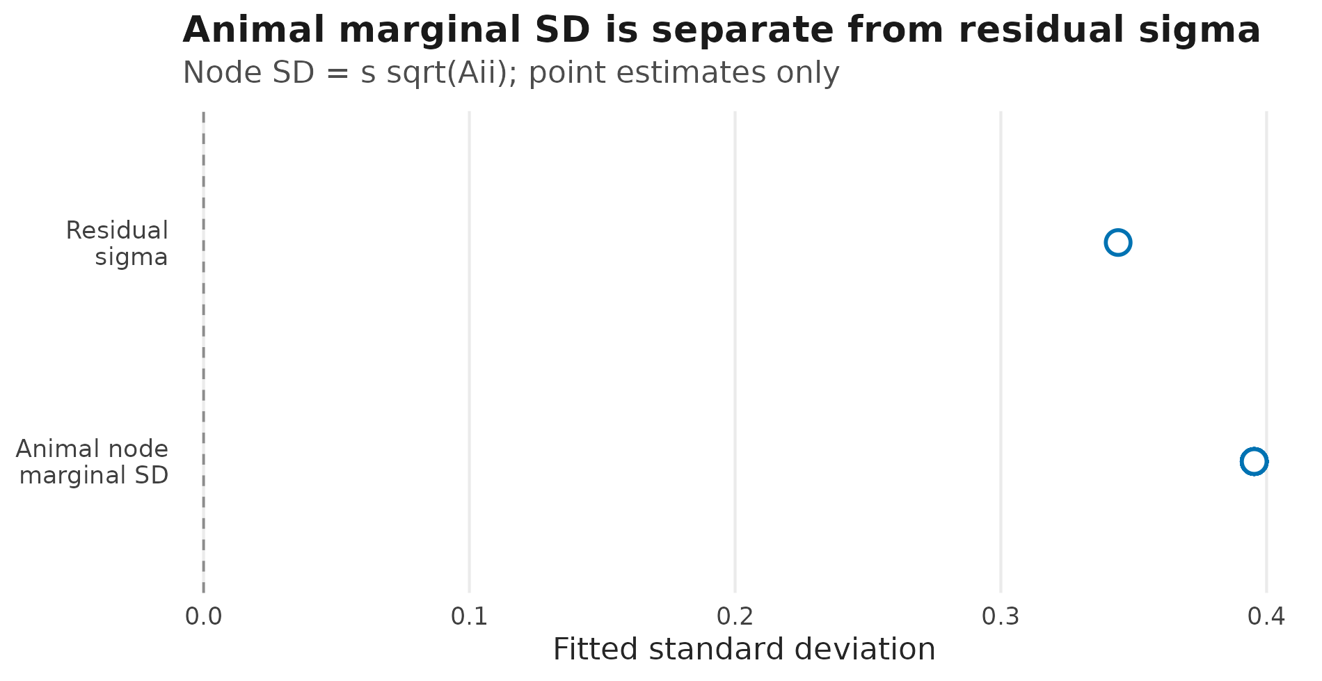
Horizontal point display comparing residual sigma with individual marginal animal standard deviations calculated as the fitted latent scale times the square root of each additive-relationship diagonal, without interval bars.

Fitted residual sigma and individual marginal animal SD point estimates s sqrt(A[i,i]) from a univariate Gaussian model. The animal q1 location-SD interval is not validated, so this comparison is point-only.

For two response means, the animal-model correlation row is a fitted latent correlation among individual additive deviations. It is not the residual rho12 correlation and it is not a raw sample correlation among observations.

animal_q2_example <- simulate_animal_q2_guide_data()
animal_q2_dat <- animal_q2_example$data
Ainv <- animal_q2_example$Ainv

fit_animal_q2_example <- drmTMB(
  bf(
    mu1 = body_size ~ climate +
      animal(1 | p | individual, Ainv = Ainv),
    mu2 = activity ~ climate +
      animal(1 | p | individual, Ainv = Ainv),
    sigma1 = ~ 1,
    sigma2 = ~ 1,
    rho12 = ~ 1
  ),
  family = c(gaussian(), gaussian()),
  data = animal_q2_dat
)

animal_q2_pairs <- corpairs(
  fit_animal_q2_example,
  level = "animal"
)
animal_q2_pairs
#>    level      group block from_dpar to_dpar   from_coef     to_coef
#> 1 animal individual     p       mu1     mu2 (Intercept) (Intercept)
#>   from_response to_response     class
#> 1     body_size    activity mean-mean
#>                                               parameter  estimate       min
#> 1 cor(mu1:(Intercept),mu2:(Intercept) | p | individual) 0.5878297 0.5878297
#>         max n_values link_estimate  link_min  link_max modelled   conf.status
#> 1 0.5878297        1     0.6743444 0.6743444 0.6743444    FALSE not_requested
#>   interval_source
#> 1   not_available

if (requireNamespace("ggplot2", quietly = TRUE)) {
  animal_q2_display <- animal_q2_pairs
  animal_q2_display$display_label <- "Animal\nmu1-mu2"

  plot_corpairs(
    animal_q2_display,
    colour = "level",
    label = "display_label",
    facet = NULL
  ) +
    ggplot2::scale_colour_manual(values = c("animal" = "#0072B2")) +
    ggplot2::scale_fill_manual(values = c("animal" = "#0072B2")) +
    animal_eye_theme() +
    ggplot2::labs(
      title = "Animal-model latent mean correlation",
      subtitle = "Point estimate only; dotted line marks zero",
      x = "Correlation estimate"
    )
}
#> Warning: No shared levels found between `names(values)` of the manual scale and the
#> data's fill values.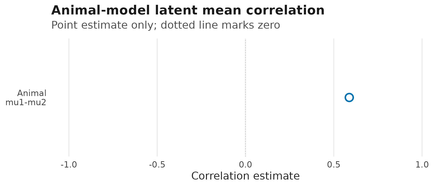

Single-row point plot for the animal-model mean-mean correlation, with a hollow point estimate to the right of the dotted zero reference line.

Animal-model intercept-only q=2 location-location point estimate from corpairs(); the dotted vertical line marks zero correlation and no interval is shown because calibration remains planned.

Boundaries

The following animal-model routes remain planned:

sparse large-pedigree precision construction;
multiple animal-model slopes such as animal(1 + x + z | individual, pedigree = pedigree);
animal-model intercept-slope correlations;
multiple or labelled residual-scale structured slopes beyond the exact A-matrix q1 animal(1 + x | individual, A = A) sigma route;
predictor-dependent animal corpair() regressions;
generic direct-SD grammar for animal-model standard deviations;
richer non-Gaussian animal structured effects: labelled covariance blocks, multiple structured slopes, structured scale routes beyond the NB2 one-slope gate, and q=2 or q=4 non-Gaussian animal covariance blocks. Exact q=1 animal gates already fit today for poisson(), nbinom2(), and beta(): Poisson, NB2, and beta mu accept an unlabelled intercept plus one independent slope; NB2 sigma accepts the same q1 intercept-plus-one-slope form; beta sigma accepts an intercept only. These rows retain their recorded point-fit/recovery tiers – trust the point estimate, not the interval.

Use the structural-dependence overview when you are choosing among animal(), phylo(), spatial(), and relmat(). Use the detailed structural-dependence tutorial when you need the current fitted examples, equations, and broader parity ladder.