Phylogenetic mixed models

Closely related species are not independent observations. They share ancestry, so a trait value carried by one species is partly inherited from the same nodes that shaped its relatives. A phylogenetic mixed model encodes that shared history as a structured random effect: a species-level deviation whose covariance is read off the tree, so that sister taxa are expected to deviate from the regression line in the same direction.

drmTMB exposes this through the phylo() term. This article explains where the covariance comes from, how to write a phylo() model for a Gaussian response, and how the same syntax carries over to non-Gaussian responses such as counts. Everything below runs at build time on a small simulated tree, so you can read the fitted numbers next to the values that generated them.

If you are choosing between animal(), phylo(), spatial(), and relmat(), read the structural-dependence overview first. When observations belong to a pair of species drawn from two different trees, read two-tree phylogenetic interactions.

The phylogenetic covariance

A phylo() term adds a vector of species-level location deviations $u$ with a mean of zero and a covariance proportional to the phylogenetic covariance matrix $A$,

$$\begin{aligned} y_{ij} &= \mathbf{x}_{ij}^\top \boldsymbol{\beta} + u_{s(i,j)} + \varepsilon_{ij}, \\ \mathbf{u} &\sim \mathcal{N}\!\left(\mathbf{0},\, \sigma_{\text{phylo}}^2\, A\right), \\ \varepsilon_{ij} &\sim \mathcal{N}\!\left(0,\, \sigma^2\right), \end{aligned}$$

where $s(i,j)$ is the species of observation $j$ in group $i$. Under a Brownian motion model of trait evolution, $A_{kl}$ is the height of the most recent common ancestor of species $k$ and $l$: the longer two species have shared an evolutionary path, the more strongly their deviations covary. For an ultrametric tree (all tips equidistant from the root), the diagonal of $A$ is constant and the off-diagonal entries are the shared root-to-ancestor path lengths.

Two standard deviations appear, and they answer different questions:

• $\sigma_{\text{phylo}}$ is the phylogenetic SD: how much species deviate from the fixed-effect prediction in a way that tracks the tree.
• $\sigma$ is the residual SD: variation among observations within a species, independent of ancestry.

Their ratio is the phylogenetic signal,

$$\lambda = \frac{\sigma_{\text{phylo}}^2}{\sigma_{\text{phylo}}^2 + \sigma^2},$$

the proportion of the random-plus-residual variance attributable to phylogeny. drmTMB reports this as a derived quantity (see below). Internally drmTMB does not invert the dense $A$. It uses the Hadfield and Nakagawa (2010) sparse phylogenetic precision (an $A^{-1}$ built from the tree’s branch lengths), which keeps the augmented-state Laplace approximation fast as the number of species grows.

A small tree with ape::rcoal()

We simulate a tree small enough to fit in a fraction of a second. ape::rcoal() draws a random ultrametric coalescent tree, which is exactly the shape phylo() expects (branch lengths present, all tips contemporaneous).

library(ape)
set.seed(2026)

n_species <- 16L
tree <- rcoal(n_species, tip.label = paste0("sp", seq_len(n_species)))

c(ultrametric = is.ultrametric(tree), n_tip = length(tree$tip.label))
#> ultrametric       n_tip 
#>           1          16

The covariance $A$ implied by this tree is available from the same internal helper the fitting code uses. We only need it here to simulate a trait with known phylogenetic structure; you never compute it by hand for a real fit.

A <- drmTMB:::drm_phylo_tip_covariance(tree)
dim(A)
#> [1] 16 16
round(A[1:4, 1:4], 3)
#>        sp7  sp11   sp2   sp5
#> sp7  1.000 0.846 0.846 0.846
#> sp11 0.846 1.000 0.850 0.850
#> sp2  0.846 0.850 1.000 0.966
#> sp5  0.846 0.850 0.966 1.000

Simulating a Gaussian trait with phylogenetic signal

We draw one species-level deviation per tip from $\mathcal{N}(0, \sigma_{\text{phylo}}^2 A)$ using a Cholesky factor of $A$, add a fixed covariate effect, and add independent residual noise. Several observations per species let the model separate the phylogenetic SD from the residual SD.

sd_phylo_true <- 0.8     # phylogenetic SD
sigma_true    <- 0.3     # residual SD
n_per_species <- 6L

# One deviation per species, correlated along the tree.
u <- as.vector(t(chol(A)) %*% rnorm(n_species, sd = sd_phylo_true))
names(u) <- tree$tip.label

species <- rep(tree$tip.label, each = n_per_species)
x <- rnorm(length(species))

# y = intercept + slope * x + phylogenetic deviation + residual noise
trait <- 0.5 - 0.4 * x + u[species] + rnorm(length(species), sd = sigma_true)

dat <- data.frame(
  trait = unname(trait),
  x = x,
  species = species
)
head(dat)
#>       trait          x species
#> 1 0.4962920  0.2284787     sp7
#> 2 0.0187960  1.1096678     sp7
#> 3 0.3970166 -0.4624204     sp7
#> 4 1.0612423 -1.6297240     sp7
#> 5 1.2921510 -1.0717278     sp7
#> 6 0.4733090  0.7681771     sp7

Fitting with phylo(1 | species)

The phylo() term goes inside the mean (mu) formula. It takes a random-effect specification, 1 | species, and the tree as tree = tree. Wrap the formulas in bf() (the drmTMB formula builder) and pass a family, exactly as for any other drmTMB model.

fit <- drmTMB(
  bf(trait ~ x + phylo(1 | species, tree = tree),
     sigma ~ 1),
  family = gaussian(),
  data = dat
)

fit$opt$convergence   # 0 indicates the optimizer converged
#> [1] 0

A few accessors return the pieces of the fit:

coef(fit, "mu")              # fixed-effect mean coefficients
#> (Intercept)           x 
#>   1.2837197  -0.4055049
fit$sdpars$mu                # phylogenetic location SD
#> phylo(1 | species) 
#>            0.77952
unique(stats::sigma(fit))    # residual SD (constant for this model)
#> [1] 0.2693226

The recovered slope (x) is close to its true value of -0.4, and the phylogenetic and residual SDs are in the neighbourhood of 0.8 and 0.3. The fixed intercept need not match the simulated 0.5: with only 16 species the species-level deviations carry a non-zero sample mean that the random effect absorbs, so the intercept and the deviations trade off. This is expected behaviour, not a fitting error – the scientifically interpretable quantities are the slope and the two SDs.

Reading the phylogenetic signal

summary() adds a derived row for the phylogenetic signal $\lambda$, alongside the random-effect and residual variances it is built from.

summary(fit)$derived[, c(
  "quantity", "estimate",
  "random_effect_variance", "residual_variance"
)]
#>                                                 quantity  estimate
#> derived:phylogenetic_signal(species) phylogenetic_signal 0.8933605
#>                                      random_effect_variance residual_variance
#> derived:phylogenetic_signal(species)              0.6076515        0.07253469

estimate is $\lambda$. A value well above zero says that, after accounting for the covariate, related species really do resemble each other more than unrelated ones. The fitted object also contains the augmented phylogenetic state used by the sparse-precision representation. To inspect only the species-tip deviations, match that state by the tree’s tip labels:

phylo_dev <- ranef(fit, "phylo_mu")
tip_dev <- phylo_dev$values[tree$tip.label]
head(tip_dev)
#>          sp7         sp11          sp2          sp5         sp13         sp15 
#> -0.655357646 -0.004477647  0.365713950  0.320016612  0.518256204  0.330854889

Uncertainty for the two SDs

Variance components have their own confint() target. The interval is on the response (SD) scale, obtained by transforming the Wald interval for the log-SD parameter. The table contains both the residual SD and the phylogenetic location SD.

confint(fit, parm = "variance_components")[, c(
  "parm", "lower", "upper", "scale"
)]
#>                       parm     lower     upper    scale
#> 1                    sigma 0.2315703 0.3132297 response
#> 2 sd:mu:phylo(1 | species) 0.5046785 1.3699263 response

A transformed log-SD interval is necessarily positive, so its lower bound should not be read as a test of a zero variance component. Use it to describe uncertainty in the magnitude of each SD. A check_drm(fit) call (not shown) reports diagnostics for the recognised phylogenetic layer.

The figure uses Confidence Eyes rather than flat interval bars. Each pale eye is the finite 95% Wald confidence region shaped on the log-SD scale: compatibility is greatest near its centre and tapers towards the endpoints. The eye is a frequentist compatibility display, not a posterior density.

vc <- confint(fit, parm = "variance_components")

phylo_sd_name <- names(fit$sdpars$mu)[
  grepl("^phylo\\(", names(fit$sdpars$mu))
]
stopifnot(length(phylo_sd_name) == 1L)

target <- c(paste0("sd:mu:", phylo_sd_name), "sigma")
interval_row <- match(target, vc$parm)
stopifnot(!anyNA(interval_row))

sd_tab <- data.frame(
  label = factor(
    c("Phylogenetic SD", "Residual SD"),
    levels = c("Residual SD", "Phylogenetic SD")
  ),
  estimate = c(
    unname(fit$sdpars$mu[[phylo_sd_name]]),
    unique(unname(stats::sigma(fit)))[1L]
  ),
  lower = vc$lower[interval_row],
  upper = vc$upper[interval_row]
)
stopifnot(
  all(is.finite(unlist(sd_tab[c("estimate", "lower", "upper")]))),
  all(sd_tab$lower > 0),
  all(sd_tab$lower <= sd_tab$estimate),
  all(sd_tab$estimate <= sd_tab$upper)
)

sd_eye <- do.call(rbind, lapply(seq_len(nrow(sd_tab)), function(i) {
  log_lower <- log(sd_tab$lower[i])
  log_upper <- log(sd_tab$upper[i])
  log_centre <- 0.5 * (log_lower + log_upper)
  log_value <- seq(log_lower, log_upper, length.out = 401L)
  half_width <- 0.5 * (log_upper - log_lower)
  height <- pmax(1 - ((log_value - log_centre) / half_width)^2, 0)
  data.frame(
    label = as.character(sd_tab$label[i]),
    value = exp(log_value),
    height = height
  )
}))
sd_eye$label <- factor(sd_eye$label, levels = levels(sd_tab$label))
sd_eye$y <- as.numeric(sd_eye$label)
sd_tab$y <- as.numeric(sd_tab$label)

ggplot2::ggplot() +
  ggplot2::geom_ribbon(
    data = sd_eye,
    ggplot2::aes(
      x = value,
      ymin = y - 0.20 * height,
      ymax = y + 0.20 * height,
      group = label
    ),
    fill = "#0072B2",
    alpha = 0.24,
    colour = NA
  ) +
  ggplot2::geom_point(
    data = sd_tab,
    ggplot2::aes(x = estimate, y = y),
    shape = 21,
    fill = "white",
    colour = "#0072B2",
    size = 3.0,
    stroke = 1.0
  ) +
  ggplot2::scale_y_continuous(
    breaks = seq_along(levels(sd_tab$label)),
    labels = levels(sd_tab$label),
    expand = ggplot2::expansion(add = 0.38)
  ) +
  ggplot2::scale_x_continuous(
    limits = c(0, NA),
    expand = ggplot2::expansion(mult = c(0, 0.04))
  ) +
  ggplot2::labs(
    x = "Standard deviation (response scale)",
    y = NULL
  ) +
  ggplot2::theme_minimal(base_size = 12.5) +
  ggplot2::theme(
    axis.line.x = ggplot2::element_line(colour = "grey40", linewidth = 0.35),
    axis.ticks.x = ggplot2::element_line(colour = "grey40", linewidth = 0.35),
    panel.grid.major.y = ggplot2::element_blank(),
    panel.grid.minor = ggplot2::element_blank(),
    axis.text.y = ggplot2::element_text(colour = "grey15")
  )

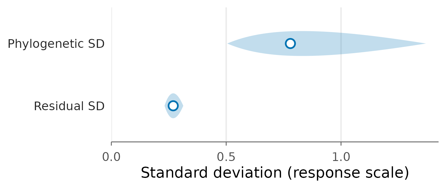
Confidence Eyes for the two response-scale SDs. Pale shapes are the default finite 95% Wald confidence regions, constructed on the log-SD scale; hollow circles are the raw fitted SDs. The default small-sample correction shifts the phylogenetic eye slightly relative to its raw estimate. The data-generating values were 0.8 and 0.3.

Non-Gaussian responses

The same phylo(1 | species, tree = tree) term works for ordinary Poisson and negative-binomial (NB2) location models. The phylogenetic deviation now acts on the linear predictor of the count mean through the log link, so related species share a baseline abundance. Two differences from the Gaussian case:

• Poisson has no residual sigma formula. NB2 instead has a modelled overdispersion sigma; its exact q1 phylogenetic sigma gate accepts an intercept plus one independent slope at recovery grade, separately from the mu field;
• the simulated deviation is built from the correlation form of $A$ (unit diagonal) scaled by the phylogenetic SD, so the SD is interpretable on the log-mean scale.

set.seed(11)

# Standardise A to a correlation matrix, then scale by the phylogenetic SD.
A_cor <- A / outer(sqrt(diag(A)), sqrt(diag(A)))
sd_phylo_count <- 0.5
u_count <- as.vector(t(chol(A_cor)) %*% rnorm(n_species)) * sd_phylo_count
names(u_count) <- tree$tip.label

species_c <- rep(tree$tip.label, each = n_per_species)
x_c <- rep(seq(-1, 1, length.out = n_per_species), times = n_species)

eta <- log(3) - 0.3 * x_c + u_count[species_c]   # log mean
count <- rpois(length(eta), lambda = exp(eta))

dat_count <- data.frame(count = count, x = x_c, species = species_c)
range(dat_count$count)
#> [1] 0 8

A Poisson fit uses the same call with family = poisson():

fit_pois <- drmTMB(
  bf(count ~ x + phylo(1 | species, tree = tree)),
  family = poisson(link = "log"),
  data = dat_count
)

fit_pois$opt$convergence
#> [1] 0
coef(fit_pois, "mu")     # log-mean intercept near log(3) ~ 1.10, slope near -0.3
#> (Intercept)           x 
#>   0.5749885  -0.3875214
fit_pois$sdpars$mu       # phylogenetic SD on the log-mean scale
#> phylo(1 | species) 
#>          0.2529665

If the counts are overdispersed relative to a Poisson, swap in nbinom2(). The NB2 family adds an overdispersion (scale) parameter while keeping the identical phylogenetic location term.

fit_nb <- drmTMB(
  bf(count ~ x + phylo(1 | species, tree = tree)),
  family = nbinom2(),
  data = dat_count
)

fit_nb$opt$convergence
#> [1] 0
fit_nb$sdpars$mu         # phylogenetic SD, NB2 mean model
#> phylo(1 | species) 
#>          0.2529666

The phylogenetic SD is reported on the log-mean (link) scale for count families, so it is not directly comparable to the Gaussian response-scale SD; compare it instead to other log-scale effects in the same model.

A larger fit, for reference

The fits above are tiny by design. For intuition about runtime on a more realistic tree, the chunk below sketches a 200-species fit. It is marked eval = FALSE so the vignette never blocks on it; the numbers in the comments are illustrative of the shape of the output, not a benchmarked claim.

set.seed(99)
big_tree <- ape::rcoal(200, tip.label = paste0("t", 1:200))
A_big <- drmTMB:::drm_phylo_tip_covariance(big_tree)
u_big <- as.vector(t(chol(A_big)) %*% rnorm(200, sd = 0.7))
names(u_big) <- big_tree$tip.label

sp <- rep(big_tree$tip.label, each = 4L)
xb <- rnorm(length(sp))
yb <- 0.2 + 0.5 * xb + u_big[sp] + rnorm(length(sp), sd = 0.3)
big <- data.frame(y = yb, x = xb, species = sp)

fit_big <- drmTMB(
  bf(y ~ x + phylo(1 | species, tree = big_tree), sigma ~ 1),
  family = gaussian(),
  data = big
)
fit_big$sdpars$mu
#> phylo(1 | species)
#>              ~0.70
# The sparse-precision path keeps this on the order of a second on a laptop;
# cost grows roughly linearly in the number of species rather than cubically.

What phylo() fits today

This is a reader-level summary of the current capability ledger. The tier words matter: diagnostic-only means a fit/extractor smoke, point-fit recovery means simulation or oracle evidence for fitted values, and inference-ready with caveats means interval evidence exists only inside the stated design. The model map gives the wider package-level boundary.

Question	Syntax	Status
Gaussian location SD	phylo(1 | species, tree = tree) or one independent slope in mu	ML intercept: inference-ready with caveats. ML intercept-plus-slope and REML intercept: point-fit recovery.
Gaussian residual-scale phylogeny	sigma ~ phylo(1 | species, tree = tree) or one independent slope	ML intercept: point-fit recovery. ML intercept-plus-slope: inference-ready with caveats. REML pure scale route: point-fit recovery.
Gaussian location and residual scale together	matching labelled phylo() terms in mu and sigma	Constant and first one-slope q=2 blocks have ML point-fit recovery; the constant REML q=2 block also has point-fit recovery.
Gaussian predictor-dependent phylogenetic SD	phylo(1 | species, tree = tree) in mu plus sd(species, level = "phylogenetic") ~ x	Fitted direct-SD route; REML admission is included in the q=1 point-fit-recovery cell. This is not a blanket interval/coverage claim.
Poisson/NB2 q1 phylogenetic mu intercept-plus-one-slope	phylo(1 + x | species, tree = tree) in mu	The exact unlabelled intercept plus one independent slope at recovery grade has point-fit recovery.
NB2 overdispersion deviations	NB2 q1 phylogenetic sigma via phylo(1 + x | species, tree = tree)	The exact unlabelled intercept-plus-one-slope route has point-fit recovery; no interval or coverage promotion.
Gamma or lognormal location SD	phylo(1 | species, tree = tree) in mu	Exact ML intercept routes have point-fit recovery; slopes, structured sigma, REML, and intervals are outside those cells.
Beta phylogenetic location-SD regression	phylo(1 | spp_id, tree = tree) in mu plus sd(spp_id, level = "phylogenetic") ~ x	Exact unlabelled q=1 ML route is inference-ready with caveats only for the validated interior-response, 1,024-species, four-replicate designs. Family sigma remains fixed-effect and $\phi = \sigma^{-2}$.
Student-t tail-weight deviations	Student-t q1 phylogenetic nu via phylo(1 | species, tree = tree)	Diagnostic-only fit/extractor evidence; not point-fit recovery.
cumulative-logit location deviations	cumulative-logit q1 phylogenetic mu via phylo(1 | species, tree = tree)	Diagnostic-only fit/extractor evidence; not point-fit recovery.
Two Gaussian means sharing phylogeny	matching phylo(1 | p | species, tree = tree) in mu1 and mu2	Intercept q=2 has ML and REML point-fit recovery; the exact ML slope-only q=2 cell is inference-ready with caveats. Read correlations with corpairs(level = "phylogenetic").
Bivariate phylogenetic location-scale blocks	matching labelled phylo() terms across mu1, mu2, sigma1, and sigma2	Exact q=2+q=2 and broader all-four cells are fitted, but their evidence ranges from diagnostic-only to point-fit recovery; they are not blanket interval/coverage claims.

When a predictor changes the phylogenetic SD itself, or when the model contains location plus two scale submodels, continue with When variance carries signal, Part II: location-scale-scale models. For the bivariate covariance layouts and the broader parity ladder, use the structural-dependence tutorial.

Anything outside these exact rows remains unpromoted, including other non-Gaussian families, additional slope/label combinations, public matrix input such as phylo(1 | species, A = A), simultaneous phylo() and spatial() layers, and structured random effects inside residual rho12.

References

Hadfield, J. D. and Nakagawa, S. (2010). General quantitative genetic methods for comparative biology: phylogenies, taxonomies and multi-trait models for continuous and categorical characters. Journal of Evolutionary Biology, 23(3), 494-508.