When variance carries signal, Part 2: location-scale-scale models

A location-scale model asks whether predictors change the expected response mu and the residual standard deviation sigma. A location-scale-scale model adds a third submodel: predictors can also change the standard deviation of a latent random effect. drmTMB writes this third submodel as sd(group) ~ predictors.

Read Part 1: location-scale models first if mu and sigma are new to you. Read Which scale are you modelling? when you need to distinguish residual SD, group-level SD, known sampling variance, and likelihood weights.

Personality, predictability, and repeatability

Suppose an exploration score is recorded repeatedly for each individual. We want to ask whether sex predicts three different features of behaviour:

1. the mean exploration score;
2. between-individual variation in expected scores; and
3. within-individual variation around each expected score.

For observation $j$ from individual $i$, write

$$\begin{aligned} y_{ij} &\sim \operatorname{Normal}(\mu_{ij}, \sigma_{e,i}^2),\\ \mu_{ij} &= \beta_0 + \beta_1\operatorname{sex}_i + b_i,\\ b_i &\sim \operatorname{Normal}(0, \sigma_{b,i}^2),\\ \log(\sigma_{e,i}) &= \gamma_0 + \gamma_1\operatorname{sex}_i,\\ \log(\sigma_{b,i}) &= \alpha_0 + \alpha_1\operatorname{sex}_i. \end{aligned}$$

Here, $\operatorname{sex}_i=0$ denotes female and $\operatorname{sex}_i=1$ denotes male. $\sigma_{b,i}$ is the between-individual SD and $\sigma_{e,i}$ is the within-individual residual SD. The matching drmTMB formula is

bf(
  exploration_score ~ sex + (1 | individual),
  sigma ~ sex,
  sd(individual) ~ sex
)

The same predictor appears in three formulas, but its coefficients answer three separate questions. Sex must be constant within each individual because it is used to model sd(individual).

Simulate and fit the three submodels

The example below gives females and males different means, between-individual SDs, and within-individual SDs. It is intentionally simple enough that the three sources of signal remain visible.

set.seed(20260721)
n_individual <- 80L
n_each <- 6L

individual_info <- data.frame(
  individual = factor(seq_len(n_individual)),
  sex = factor(
    rep(c("female", "male"), each = n_individual / 2),
    levels = c("female", "male")
  )
)

mean_by_sex <- c(female = 0.35, male = 0.70)
between_sd_by_sex <- c(female = 0.65, male = 0.40)
within_sd_by_sex <- c(female = 0.35, male = 0.60)

individual_effect <- stats::rnorm(
  n_individual,
  sd = between_sd_by_sex[individual_info$sex]
)

personality <- individual_info[rep(seq_len(n_individual), each = n_each), ]
personality$exploration_score <-
  mean_by_sex[personality$sex] +
  individual_effect[as.integer(personality$individual)] +
  stats::rnorm(
    nrow(personality),
    sd = within_sd_by_sex[personality$sex]
  )

fit_personality <- drmTMB(
  bf(
    exploration_score ~ sex + (1 | individual),
    sigma ~ sex,
    sd(individual) ~ sex
  ),
  family = gaussian(),
  data = personality
)

round(coef(fit_personality, "mu"), 3)
#> (Intercept)     sexmale 
#>       0.461       0.205
round(coef(fit_personality, "sigma"), 3)
#> (Intercept)     sexmale 
#>      -1.042       0.595
round(coef(fit_personality, "sd(individual)"), 3)
#> (Intercept)     sexmale 
#>      -0.407      -0.669

The sigma and sd(individual) coefficients use log-SD links. For example, exponentiating the male coefficient from sigma gives the male-to-female ratio of within-individual SDs. Exponentiating the corresponding sd(individual) coefficient gives the male-to-female ratio of between-individual SDs.

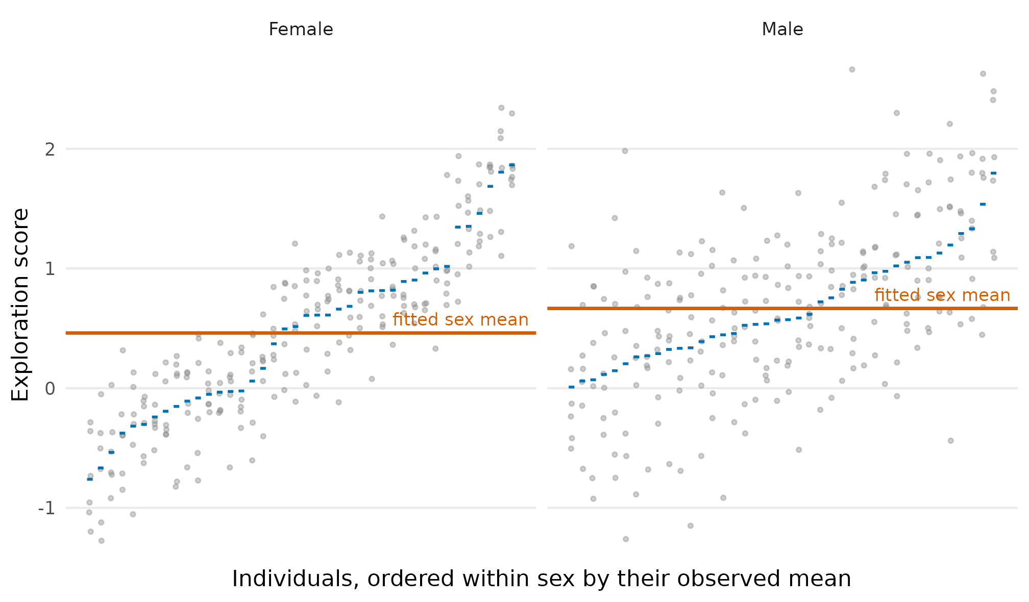
Repeated exploration scores for females and males. Grey points are observations, blue ticks are individual means, and the vermillion line is the fitted sex-specific mean. The spread of individual means represents between-individual variation; scatter around each individual mean represents within-individual variation. Both panels use the same vertical scale.

Read the fitted scales and calculate repeatability

Predictions with newdata are population-level values. They give the three fitted quantities for each sex directly on their natural scales.

sex_grid$mean_score <- predict(
  fit_personality, newdata = sex_grid, dpar = "mu"
)
sex_grid$between_individual_sd <- predict(
  fit_personality, newdata = sex_grid, dpar = "sd(individual)"
)
sex_grid$within_individual_sd <- predict(
  fit_personality, newdata = sex_grid, dpar = "sigma"
)

sex_grid$repeatability <- with(
  sex_grid,
  between_individual_sd^2 /
    (between_individual_sd^2 + within_individual_sd^2)
)

repeatability_table <- sex_grid[c(
  "sex",
  "mean_score",
  "between_individual_sd",
  "within_individual_sd",
  "repeatability"
)]
repeatability_table[-1] <- lapply(
  repeatability_table[-1],
  round,
  digits = 3
)
repeatability_table
#>      sex mean_score between_individual_sd within_individual_sd repeatability
#> 1 female      0.461                 0.665                0.353         0.781
#> 2   male      0.666                 0.341                0.639         0.221

In behavioural ecology, this intraclass correlation is usually called repeatability. For sex $s$,

$$R_s = \frac{\sigma_{b,s}^2} {\sigma_{b,s}^2 + \sigma_{e,s}^2}.$$

Repeatability is derived from the two fitted scale submodels; it is not a fourth formula. The calculation above is a point estimate. It does not supply an uncertainty interval for this nonlinear ratio.

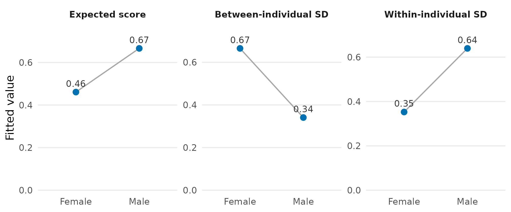
Model-implied values for females and males. Panels show the expected exploration score, between-individual SD from sd(individual), and within-individual residual SD from sigma. Lines aid comparison and are not uncertainty intervals.

A short phylogenetic extension

The same three-part logic applies when the latent location effect follows a phylogeny. Start from the familiar constant-scale model

$$\begin{aligned} y_i &= \mu_i + a_i + e_i,\\ \mu_i &= \beta_0 + \beta_1 T_i,\\ \mathbf a &\sim \operatorname{MVN}(\mathbf 0, \sigma_a^2 A),\\ e_i &\sim \operatorname{Normal}(0, \sigma_e^2), \end{aligned}$$

where $A$ is the phylogenetic correlation matrix and $T_i$ is temperature. A location-scale-scale extension lets both SDs change linearly with temperature:

$$\log(\sigma_{e,i}) = \gamma_0 + \gamma_1 T_i, \qquad \log(\sigma_{a,i}) = \alpha_0 + \alpha_1 T_i.$$

The matching syntax is deliberately simple:

fit_phylo_lss <- drmTMB(
  bf(
    trait ~ temperature + phylo(1 | species, tree = tree),
    sigma ~ temperature,
    sd(species, level = "phylogenetic") ~ temperature
  ),
  family = gaussian(),
  data = dat
)

Formula	Model quantity	Interpretation
trait ~ temperature + phylo(...)	$\mu_i$ and $a_i$	expected trait and phylogenetically correlated location deviation
sigma ~ temperature	$\sigma_{e,i}$	independent SD
sd(species, level = "phylogenetic") ~ temperature	$\sigma_{a,i}$	SD of the phylogenetic location deviation

The scalar covariance $\sigma_a^2 A$ is the constant-SD starting point. The third formula generalizes it by allowing the phylogenetic-effect SD to vary among species with temperature. The older formula spelling sd_phylo(species) ~ temperature is soft-deprecated; fitted objects retain the output label sd_phylo(species) for extractor compatibility.

With repeated observations within species, sigma is the within-species residual SD. With one response row per species, it is the independent non-phylogenetic species-level deviation. It should not automatically be described as measurement error.

Current boundaries

• Ordinary sd(group) ~ predictors is implemented for distinct unlabelled Gaussian mu random intercepts. The matching (1 | group) term must appear in the location formula, and scale predictors must be constant within group.
• sd(group, level = "phylogenetic") ~ predictors targets the location phylogenetic effect introduced by phylo() in mu; predictors must be constant within species.
• This article teaches the Gaussian route. Check narrow non-Gaussian cells in What can I fit today? rather than generalizing from it.
• Random effects on the right-hand side of an sd() formula and generic direct-SD levels for spatial(), animal(), and relmat() remain separate implementation and validation questions.
• Use check_drm(), inspect the terminal gradient and Hessian diagnostics, and retain failed fits. A clean optimizer code alone does not establish that every SD surface is well identified.

For broader phylogenetic syntax, continue to Phylogenetic mixed models. For prediction tables and the distinction between sigma and sd(group), return to Which scale are you modelling?.

Reference

Nakagawa, S., Mizuno, A., Williams, C., Lagisz, M., Yang, Y., and Drobniak, S. M. (2025). Quantifying macro-evolutionary patterns of trait mean and variance with phylogenetic location-scale models. Methods in Ecology and Evolution. doi:10.1111/2041-210X.70160.