Known-matrix relatedness with relmat

Use relmat() when the dependence is among latent group-level deviations and the matrix is already known. The matrix can be a covariance, a correlation, or an inverse covariance/precision matrix. The common case is a correlation-like matrix among lines, strains, plots, populations, or experimental units:

u_id ~ N(0, sd_relmat^2 K)
y_i  = mu_i + u_id[i] + error_i

If the natural input is a precision matrix, use Q instead:

u_id ~ N(0, sd_relmat^2 Q^-1)

This is a higher-level random-effect structure. It is not the same as known sampling covariance among observed effect-size estimates; that observation-level matrix belongs to the meta-analysis route with meta_V(V = V).

When is relmat() the right tool?

Use relmat() only after the named biological or spatial route is not the better description. It is the general fallback for a matrix you already have, so reach for it once the structural-dependence overview has ruled out the named routes.

Situation	Use	Why
Genomic or marker-based similarity among inbred lines, strains, or cultivars	relmat(1 | line, K = G)	G is often a correlation or genomic relationship matrix. The fitted SD turns it into the latent covariance sd_relmat^2 G.
A lab, assay, or ecological kernel among experimental units	relmat(1 | unit, K = K_unit)	The matrix says which unit-level deviations should be similar, but it is not a pedigree, species tree, or coordinate-spatial surface.
A precomputed inverse relatedness matrix from another tool	relmat(1 | id, Q = Q_id)	The natural object is already precision-like, so drmTMB does not need to invert a dense covariance matrix.
A graph, network, river, areal, or custom Gaussian Markov random-field precision that was built and checked outside drmTMB	relmat(1 | node, Q = Q_node)	The scientific structure is a latent node-level field with a known precision, but it is not the current coordinate spatial() route.

Do not use relmat() just because you have any covariance matrix. If the matrix is known sampling covariance for observed estimates, use meta_V(V = V). If the matrix is additive relatedness from a pedigree or animal model, use animal(). If it comes from an ultrametric species tree, use phylo(). If coordinates define the dependence, use spatial().

Choosing K or Q

Use K when the matrix is easiest to interpret as relatedness, covariance, or correlation. A correlation matrix with diagonal 1 is usually the clearest input: the fitted sd_relmat then controls the variance scale of the latent deviations. A covariance matrix with non-unit diagonal is also allowed, but then the diagonal scale is part of the known structure.

Use Q when the matrix is easiest to interpret as an inverse covariance or precision. This is common when another model, pedigree engine, graph model, or Gaussian Markov random-field construction gives a sparse precision matrix. In that case the latent covariance is proportional to solve(Q), but the model can work with Q directly.

Two concrete examples

Suppose G is a marker-derived genomic relationship matrix among experimental lines. The scientific question is whether lines that are genomically similar also have similar unexplained deviations in seed mass:

fit_grm <- drmTMB(
  bf(seed_mass ~ temperature + relmat(1 | line, K = G), sigma ~ temperature),
  data = dat,
  family = gaussian()
)

Here G can be a correlation matrix. fit_grm$sdpars$mu reports the fitted structured SD scale s, so the latent covariance is s^2 G and line i has marginal SD s sqrt(G[i, i]). Thus s is a line-level marginal SD only when the corresponding diagonal entry of G is one. This is not known sampling error; it is latent among-line structure left after the fixed effects.

Now suppose Q_river is a positive-definite precision matrix for sites on a river network, built outside drmTMB from an adjacency or flow model. The scientific question is whether nearby or connected sites have similar latent condition deviations:

fit_river <- drmTMB(
  bf(condition ~ treatment + relmat(1 | reach, Q = Q_river), sigma ~ 1),
  data = dat,
  family = gaussian()
)

This is a good Q example because the natural object is already an inverse covariance. If C = solve(Q_river), the model estimates the fitted structured scale s, the latent covariance is s^2 C, and reach i has marginal SD s sqrt(C[i, i]). The known precision controls the pattern of similarity across reaches; s is not a common site-level marginal SD unless diag(C) is one.

What is fitted today

Question	Syntax	Status
Does one Gaussian response have deviations structured by a user-supplied latent covariance or precision matrix?	relmat(1 | id, K = K) or relmat(1 | id, Q = Q) in mu	Fitted first slice. K is a covariance matrix; Q is a precision matrix.
Does one numeric fixed-effect slope also have known-matrix deviations?	relmat(1 + x | id, K = K) or relmat(1 + x | id, Q = Q) in mu	Fitted first univariate one-slope slice with independent intercept and slope fields. Additional structured-slope layouts outside the exact fitted bivariate ledger cells and intercept-slope correlations remain planned.
Does a one-response Gaussian model have known-matrix residual-scale deviations?	relmat(1 | id, Q = Q) in sigma, alone or matching the mu term; relmat(1 + x | id, K = K) for the exact one-slope route	The residual-scale intercept is fitted. The exact K/Q q1 sigma one-slope route is fitted and inference-ready with caveats under raw uncorrected log-SD Wald-z intervals; profile is diagnostic-only at g = 8. Matching univariate mu and sigma relmat() intercepts estimate one known-matrix mean-scale correlation. Broader K/Q bridge claims, additional multiple or labelled sigma-slope layouts outside the exact fitted bivariate ledger cells, and structured slope correlations remain planned.
Do two Gaussian response means share a known-matrix latent correlation?	matching labelled relmat(1 | p | id, K = K) or relmat(1 | p | id, Q = Q) terms in mu1 and mu2	ML fits both representations. Native REML has point_fit_recovery evidence only for the exact supplied-K, location-intercept cell with constant residual formulas, complete pairs, unit weights, and no other model layer. corpairs(level = "relmat") reports the latent relatedness correlation separately from residual rho12. Q remains ML-only for this bivariate route.
Does the known-matrix layer link means and residual scales across two responses?	the same labelled relmat(1 | p | id, Q = Q) term in mu1, mu2, sigma1, and sigma2	Fitted first q=4 location-scale slice. corpairs(level = "relmat") reports six constant latent relatedness correlations; profile intervals for those derived correlations remain unavailable.
Does the known-matrix layer change multiple slopes or a predictor-dependent correlation?	examples such as relmat(1 + x + z | id, K = K) or relmat() corpair() formulas	Planned. These routes need matrix validation, diagnostics, recovery tests, interval targets, and examples before use.

Use animal() when the matrix is additive relatedness for individual animal models. Use phylo() when the matrix comes from a species tree and the tree route is available. Use spatial() when the structure is induced by sampling coordinates. Use relmat() for validated latent matrices that do not belong to those named routes.

Start with the smallest useful model

For one response, start with the fitted location-intercept route:

fit_relmat <- drmTMB(
  y ~ treatment + relmat(1 | line, K = K),
  data = dat,
  family = gaussian()
)

For the exact Arc 1a REML route, keep sigma ~ 1, use an unlabelled intercept or independent intercept-plus-one-numeric-slope shape, and set REML = TRUE:

fit_relmat_reml <- drmTMB(
  bf(
    y ~ x + relmat(1 + x | line, K = K),
    sigma ~ 1
  ),
  data = dat,
  family = gaussian(),
  REML = TRUE
)

The multi-seed campaign used the K representation shown here, with n_each = 20 and exactly M = {8, 16, 32} relatedness levels. Q has deterministic representation-parity evidence only, not multi-seed campaign coverage. Those Arc 1a domains do not admit slope-only, labelled, multiple-slope, scale-side, bivariate, or non-Gaussian REML routes. The separate exact bivariate supplied-K exception is shown next.

For two responses under REML, build one named covariance matrix whose rows and columns exactly match the factor levels, then use the same matrix and block label in mu1 and mu2. This complete example constructs the data and a dense correlation matrix rather than leaving either object undefined:

set.seed(20260715)
line_levels <- paste0("line_", seq_len(10))
line <- factor(rep(line_levels, each = 6), levels = line_levels)
treatment <- rep(rep(c(0, 1), each = 3), length(line_levels))
index <- seq_along(line_levels)
K <- outer(index, index, function(i, j) 0.4^abs(i - j))
dimnames(K) <- list(line_levels, line_levels)
L <- t(chol(K))
z1 <- rnorm(length(line_levels))
z2 <- 0.35 * z1 + sqrt(1 - 0.35^2) * rnorm(length(line_levels))
u1 <- setNames(as.vector(L %*% z1) * 0.8, line_levels)
u2 <- setNames(as.vector(L %*% z2) * 0.65, line_levels)
e1 <- rnorm(length(line))
e2 <- -0.2 * e1 + sqrt(1 - 0.2^2) * rnorm(length(line))
dat <- data.frame(
  trait1 = 0.3 + 0.5 * treatment + u1[line] + 0.3 * e1,
  trait2 = -0.2 - 0.25 * treatment + u2[line] + 0.35 * e2,
  treatment = treatment,
  line = line
)

fit_relmat_q2_reml <- drmTMB(
  bf(
    mu1 = trait1 ~ treatment + relmat(1 | p | line, K = K),
    mu2 = trait2 ~ treatment + relmat(1 | p | line, K = K),
    sigma1 = ~ 1,
    sigma2 = ~ 1,
    rho12 = ~ 1
  ),
  data = dat,
  family = biv_gaussian(),
  REML = TRUE
)
corpairs(fit_relmat_q2_reml, level = "relmat")
rho12(fit_relmat_q2_reml)

corpairs() reports the fitted latent known-matrix correlation among line or unit-level location deviations. rho12() reports the residual correlation between responses after fixed effects and random effects have been included. The REML claim stops at point_fit_recovery: intervals and coverage remain unvalidated.

The precision representation remains available for the established ML q2 route, not for this bivariate REML exception:

Q <- solve(K)
fit_relmat_q2_ml <- drmTMB(
  bf(
    mu1 = trait1 ~ treatment + relmat(1 | p | line, Q = Q),
    mu2 = trait2 ~ treatment + relmat(1 | p | line, Q = Q),
    sigma1 = ~ 1,
    sigma2 = ~ 1,
    rho12 = ~ 1
  ),
  data = dat,
  family = biv_gaussian(),
  REML = FALSE
)

For reports, keep this intercept-only q=2 known-matrix correlation point-only. The profile mechanism is callable, but interval calibration and coverage are still planned for this row:

relmat_pairs <- corpairs(fit_relmat_q2_reml, level = "relmat")
plot_corpairs(relmat_pairs)

That plot should be read as a latent known-matrix correlation display, not as a residual rho12 plot. Do not add an interval eye until this exact row has validated interval evidence. The q=4 rows below are also point-only: current q=4 relmat() correlations are derived rows.

When the scientific question is whether known-matrix deviations in means and residual scales covary, use the same labelled relmat() term in all four bivariate endpoint formulas:

fit_relmat_q4 <- drmTMB(
  bf(
    mu1 = trait1 ~ treatment +
      relmat(1 | p | line, Q = Q),
    mu2 = trait2 ~ treatment +
      relmat(1 | p | line, Q = Q),
    sigma1 = ~ treatment +
      relmat(1 | p | line, Q = Q),
    sigma2 = ~ treatment +
      relmat(1 | p | line, Q = Q)
  ),
  data = dat,
  family = biv_gaussian()
)
corpairs(fit_relmat_q4, level = "relmat")

The q=4 path is constant across levels and responses: it estimates four latent known-matrix endpoint scale parameters and six latent correlations. Each endpoint’s level-specific marginal SD also includes the corresponding known diagonal multiplier. This is not a direct-SD model and it does not make the residual correlation rho12 known-matrix structured.

What to inspect

After fitting, inspect the relatedness layer before interpreting it:

Output	Use
check_drm(fit)	Confirm the relmat() layer was recognized and review matrix/replication diagnostics.
fit$sdpars$mu	Read the fitted latent known-matrix scale s; level i has marginal SD s sqrt(K[i, i]).
ranef(fit, "relmat_mu")	Inspect conditional deviations on the fitted relatedness layer.
summary(fit)$covariance	Check how the relmat() SD or q=2 correlation is reported beside other covariance layers.
profile_targets(fit)	See which relatedness SD or q=2 correlation targets can be profiled directly; q=4 correlations are derived-only in the first slice.
corpairs(fit, level = "relmat")	Read the fitted q=2 relatedness mean-mean correlation, or the six q=4 relatedness endpoint correlations when the model has the all-four block.

Rendered checks

The examples below keep the matrix, standard deviations, and correlation row in separate visual grammars. The known matrix is raw input structure, not uncertainty. The latent relmat scale s uses the validated default location-axis bias-corrected small-sample-t Wald channel for the exact K-matrix q1 row. The plot multiplies its point and interval endpoints by each known sqrt(K[i, i]) before comparing node marginal SDs with residual sigma, whose interval uses its ordinary Wald route. The intercept-only q=2 relatedness correlation is a point estimate with a dotted zero line. Its profile mechanics are diagnostic-only; interval calibration and coverage are still planned.

relmat_example <- simulate_relmat_guide_data()
relmat_dat <- relmat_example$data
K <- relmat_example$K
Q <- relmat_example$Q

fit_relmat <- drmTMB(
  bf(
    seed_mass ~ temperature + treatment + relmat(1 | line, K = K),
    sigma ~ 1
  ),
  family = gaussian(),
  data = relmat_dat
)

if (requireNamespace("ggplot2", quietly = TRUE)) {
  relmat_matrix <- relatedness_heatmap_data(K)

  ggplot2::ggplot(
    relmat_matrix,
    ggplot2::aes(column, row, fill = relatedness)
  ) +
    ggplot2::geom_tile() +
    ggplot2::coord_equal() +
    ggplot2::scale_fill_gradientn(
      colours = c("#F7FCF5", "#C7E9C0", "#74C476", "#006D2C"),
      name = "Known\nrelatedness"
    ) +
    relmat_guide_theme() +
    ggplot2::theme(
      axis.text = ggplot2::element_blank(),
      axis.ticks = ggplot2::element_blank(),
      panel.grid = ggplot2::element_blank()
    ) +
    ggplot2::labs(
      title = "Known-matrix input structure",
      subtitle = "Validated relatedness among experimental lines",
      x = "Line",
      y = "Line"
    )
}

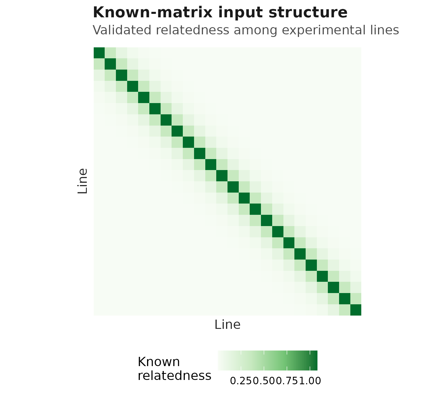
Known relatedness matrix used by the relmat() example; this heatmap shows the supplied latent structure, not model-estimated uncertainty.

if (requireNamespace("ggplot2", quietly = TRUE)) {
  relmat_ci <- confint(fit_relmat, parm = "variance_components")
  node_multiplier <- sqrt(diag(K))
  relmat_sd <- relmat_ci[c(1, rep(2, length(node_multiplier))), , drop = FALSE]
  relmat_sd$estimate <- c(
    unname(exp(coef(fit_relmat, "sigma")["(Intercept)"])),
    unname(fit_relmat$sdpars$mu["relmat(1 | line)"]) * node_multiplier
  )
  relmat_sd$lower[-1] <- relmat_sd$lower[-1] * node_multiplier
  relmat_sd$upper[-1] <- relmat_sd$upper[-1] * node_multiplier
  relmat_sd$label <- c(
    "Residual\nsigma",
    rep("relmat node\nmarginal SD", length(node_multiplier))
  )

  ggplot2::ggplot(relmat_sd, ggplot2::aes(y = label)) +
    ggplot2::geom_vline(
      xintercept = 0,
      linewidth = 0.45,
      linetype = "dashed",
      colour = "grey55"
    ) +
    ggplot2::geom_errorbar(
      ggplot2::aes(xmin = lower, xmax = upper),
      width = 0,
      linewidth = 1.1,
      colour = "#009E73"
    ) +
    ggplot2::geom_point(
      ggplot2::aes(x = estimate),
      shape = 21,
      size = 3.5,
      stroke = 1,
      fill = "white",
      colour = "#009E73"
    ) +
    ggplot2::scale_x_continuous(
      expand = ggplot2::expansion(mult = c(0.02, 0.05))
    ) +
    relmat_eye_theme() +
    ggplot2::labs(
      title = "Known-matrix marginal SD is separate from residual sigma",
      subtitle = "Node SD = s sqrt(Kii); bars are transformed 95% Wald intervals",
      x = "Fitted standard deviation",
      y = NULL
    )
}

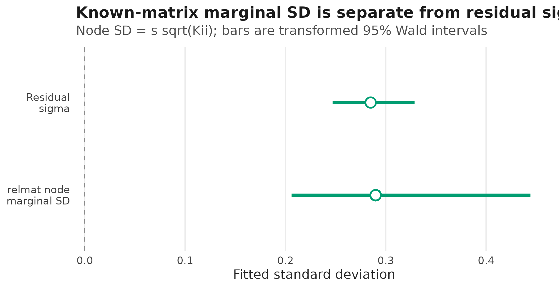
Fitted residual sigma and level-specific known-matrix marginal SDs s sqrt(K[i,i]) from a univariate Gaussian relmat() model. Points and bars are response-scale estimates with 95% Wald intervals transformed by the known diagonal multipliers.

For two response means, the known-matrix row is a fitted latent correlation among line-level deviations. It is not residual rho12 and it is not a raw correlation among observations.

relmat_q2_example <- simulate_relmat_q2_guide_data()
relmat_q2_dat <- relmat_q2_example$data
K <- relmat_q2_example$K

fit_relmat_q2_example <- drmTMB(
  bf(
    mu1 = seed_mass ~ age + sex +
      relmat(1 | p | line, K = K),
    mu2 = plant_height ~ age + sex +
      relmat(1 | p | line, K = K),
    sigma1 = ~ 1,
    sigma2 = ~ 1,
    rho12 = ~ 1
  ),
  family = biv_gaussian(),
  data = relmat_q2_dat,
  REML = TRUE
)

relmat_q2_pairs <- corpairs(
  fit_relmat_q2_example,
  level = "relmat"
)
relmat_q2_pairs
#>    level group block from_dpar to_dpar   from_coef     to_coef from_response
#> 1 relmat  line     p       mu1     mu2 (Intercept) (Intercept)     seed_mass
#>    to_response     class                                       parameter
#> 1 plant_height mean-mean cor(mu1:(Intercept),mu2:(Intercept) | p | line)
#>   estimate      min      max n_values link_estimate  link_min  link_max
#> 1 0.328678 0.328678 0.328678        1     0.3413458 0.3413458 0.3413458
#>   modelled   conf.status interval_source
#> 1    FALSE not_requested   not_available

if (requireNamespace("ggplot2", quietly = TRUE)) {
  relmat_q2_display <- relmat_q2_pairs
  relmat_q2_display$display_label <- "relmat\nmu1-mu2"

  plot_corpairs(
    relmat_q2_display,
    colour = NULL,
    label = "display_label",
    facet = NULL
  ) +
    relmat_eye_theme() +
    ggplot2::labs(
      title = "Known-matrix latent mean correlation",
      subtitle = "Point estimate only; dotted line marks zero",
      x = "Correlation estimate"
    )
}

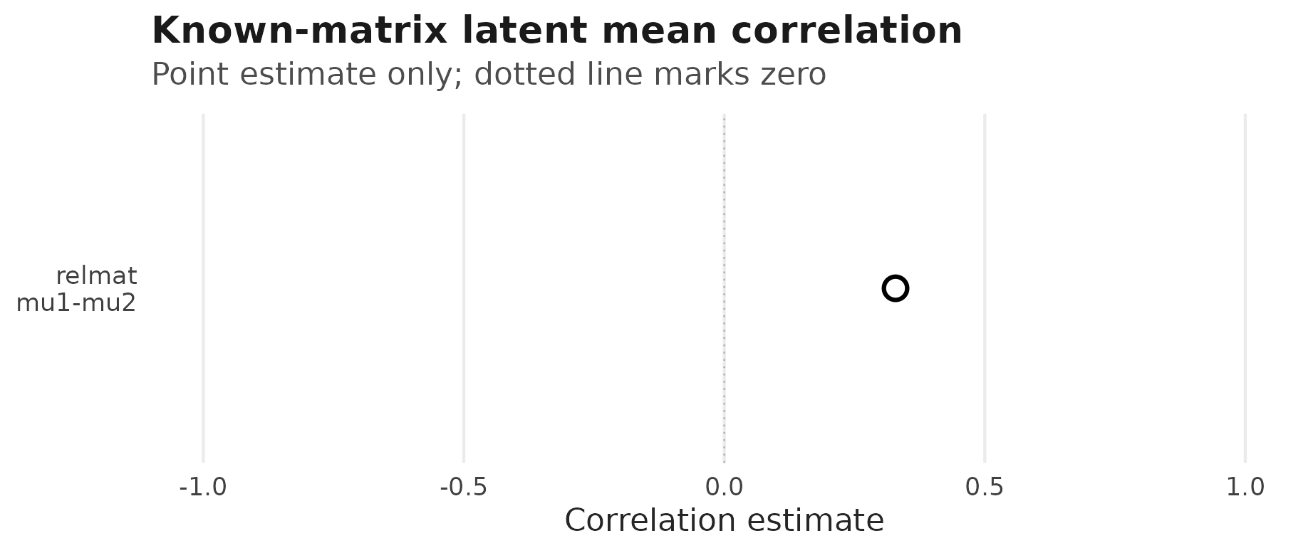
relmat() intercept-only q=2 location-location point estimate from corpairs(); the dotted vertical line marks zero correlation and no interval is shown because calibration remains planned.

Boundaries

The following relmat() routes remain planned:

• multiple structured slopes such as relmat(1 + x + z | id, K = K);
• known-matrix intercept-slope correlations;
• multiple or labelled residual-scale structured slopes beyond the exact q1 relmat(1 + x | id, K = K) sigma route;
• predictor-dependent relmat() corpair() regressions;
• generic direct-SD grammar for known-matrix standard deviations;
• bivariate relmat REML with Q, slopes, q4 or larger blocks, scale-side terms, extra random effects, incomplete pairs, non-unit weights, or nonconstant sigma1, sigma2, or rho12 formulas;
• non-Gaussian known-matrix structured effects beyond the first recovery-grade gates noted below.

Several non-Gaussian families already fit a first q1 unlabelled relmat() structured gate with route-specific evidence. The recovery-grade routes support point estimates but are not coverage-validated: Gamma(), poisson(), and nbinom2() each accept a mu intercept plus one independent slope; nbinom2() also accepts a sigma intercept plus one independent slope. Separately, truncated_nbinom2() (with its hurdle NB2 alias) accepts a diagnostic-only intercept-only hu gate. Use that route only to confirm fit/extractor feasibility; it does not establish point-estimate recovery. The beta() family and the families with no structured layer still reject relmat().

Known sampling covariance is a different model layer, not a separate relatedness route. If the matrix describes known observation-level uncertainty for effect-size estimates, use meta_V(V = V) – deprecated meta_known_V(V = V) remains a compatibility alias – and the meta-analysis documentation instead of relmat().

Use the structural-dependence overview when you are choosing among animal(), phylo(), spatial(), and relmat(). Use the detailed structural-dependence tutorial when you need the current fitted examples, equations, and broader parity ladder.