Model-conditional centile chart

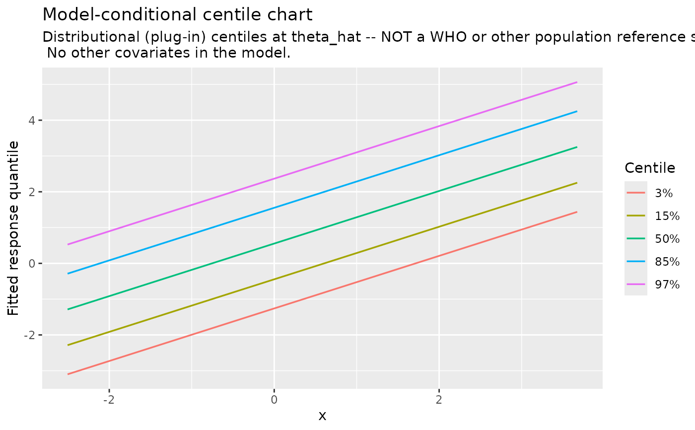
centile_chart() draws fitted response centile curves against one covariate, holding every other predictor at a reference value (numeric predictors at their fitted mean, factors at their first fitted level; see prediction_grid()). Each curve is predict(object, newdata = grid, type = "quantile", prob = p) for one p in prob.

Usage

centile_chart(object, covariate, prob = c(0.03, 0.15, 0.5, 0.85, 0.97), ...)

# S3 method for class 'drmTMB'
centile_chart(
  object,
  covariate,
  prob = c(0.03, 0.15, 0.5, 0.85, 0.97),
  dpar = NULL,
  n = 100L,
  ...
)

Arguments

object

A drmTMB fit.

covariate

Character scalar naming the predictor to vary.

prob

Numeric vector of probabilities in (0, 1) giving the centiles to draw.

...

Reserved for future options.

dpar

Distributional parameter identifying the response; see predict.drmTMB(). If NULL, the first fitted distributional parameter is used (for bivariate biv_gaussian fits, dpar selects the response – see predict.drmTMB()'s Details for the marginal-only scope).

n

Number of grid points spanning covariate's fitted range; passed to prediction_grid().

Value

A ggplot object.

Details

centile_chart() is a MODEL-CONDITIONAL summary at predict_parameters()'s fixed-effect, population-level parameter estimates theta_hat – it is not a WHO-style or other population reference standard. The reference values every non-focal covariate is held at are reported in the plot subtitle so a reader is not left guessing what "conditional" means here.

See also

predict.drmTMB(), prediction_grid()

Examples

set.seed(20260712)
n <- 60
x <- stats::rnorm(n)
dat <- data.frame(y = 0.5 + 0.8 * x + stats::rnorm(n), x = x)
fit <- drmTMB(bf(y ~ x, sigma ~ 1), family = gaussian(), data = dat)
if (requireNamespace("ggplot2", quietly = TRUE)) {
  centile_chart(fit, covariate = "x")
}