When group variation changes with a predictor

This guide shows how to ask whether groups differ in their typical spread, and whether that spread changes with a group-level predictor. It starts with synthetic Bernoulli and Poisson data, then uses a Gamma model for positive responses from related groups. The data-generating values are known. The Bernoulli and Poisson models estimate a random-intercept standard deviation; they do not estimate a separate residual sigma. The Gamma example separates its conditional response spread from the scale of its latent group effects.

The model

For a binary response, the group effect shifts the log odds:

\[ \begin{aligned} Y_{ig} \mid b_g &\sim \operatorname{Bernoulli}(p_{ig}), \\ \operatorname{logit}(p_{ig}) &= \beta_0 + \beta_1 x_{ig} + b_g, \\ b_g &\sim \operatorname{Normal}(0, s_g^2), \\ \log(s_g) &= \alpha_0 + \alpha_1 w_g. \end{aligned} \]

For counts, the same random effect shifts the log expected count:

\[ \begin{aligned} Y_{ig} \mid b_g &\sim \operatorname{Poisson}(\mu_{ig}), \\ \log(\mu_{ig}) &= \beta_0 + \beta_1 x_{ig} + b_g, \\ b_g &\sim \operatorname{Normal}(0, s_g^2), \\ \log(s_g) &= \alpha_0 + \alpha_1 w_g. \end{aligned} \]

Here, x varies among observations and w is constant within each group. The fixed-effect coefficient for x describes a change in the mean predictor. The coefficient alpha_1 describes how the spread of group effects changes: because the log link is used for s_g, a one-unit increase in w multiplies the random-intercept SD by exp(alpha_1). It does not multiply the variance by that amount; the variance ratio is exp(2 * alpha_1).

The R formula keeps those questions separate. For example, y ~ x + (1 | group) models the response predictor, while sd(group) ~ w models the SD of the latent group intercept. The group-level predictor must have one value per group; a within-group predictor belongs in the mean formula in this scalar-intercept example. More general random- regression models can use within-group predictors to define random slopes; that is a different model structure from the intercept-only examples here.

Make two small synthetic data sets

The examples use 60 groups with 10 observations per group. The two values of w differ by one unit, so exponentiating its fitted coefficient gives the high-w to low-w random-intercept SD ratio.

set.seed(20261017)
n_group <- 60L
n_per_group <- 10L
group_info <- data.frame(
  group = factor(seq_len(n_group)),
  w = rep(c(-0.5, 0.5), each = n_group / 2)
)
group_index <- rep(seq_len(n_group), each = n_per_group)

bernoulli_data <- group_info[group_index, , drop = FALSE]
bernoulli_data$x <- stats::rnorm(nrow(bernoulli_data))
bernoulli_b <- exp(-0.4 + 0.45 * group_info$w) *
  stats::rnorm(n_group)
bernoulli_data$y <- stats::rbinom(
  nrow(bernoulli_data),
  size = 1,
  prob = stats::plogis(
    -0.25 + 0.5 * bernoulli_data$x + bernoulli_b[group_index]
  )
)

poisson_data <- group_info[group_index, , drop = FALSE]
poisson_data$x <- stats::rnorm(nrow(poisson_data))
poisson_b <- exp(-0.4 + 0.45 * group_info$w) *
  stats::rnorm(n_group)
poisson_data$y <- stats::rpois(
  nrow(poisson_data),
  lambda = exp(-0.2 + 0.3 * poisson_data$x + poisson_b[group_index])
)

Each data set has a binary group-level predictor and an observation-level predictor. The latent effects are generated with an SD that increases with w. The response-specific intercept and slope values differ between the two examples, so the Bernoulli and Poisson fits are independent illustrations.

Fit a Bernoulli model

The Bernoulli likelihood has no free residual sigma. The fitted random intercept is on the logit scale, and sd(group) ~ w describes its group-level standard deviation on that same latent scale.

fit_bernoulli <- drmTMB(
  bf(y ~ x + (1 | group), sd(group) ~ w),
  family = stats::binomial(link = "logit"),
  data = bernoulli_data
)

bernoulli_checks <- check_drm(fit_bernoulli)
data.frame(check = bernoulli_checks$check, status = bernoulli_checks$status)
#>                           check status
#> 1         optimizer_convergence     ok
#> 2            convergence_status     ok
#> 3              optimizer_budget     ok
#> 4              finite_objective     ok
#> 5         logsigma_clamp_active     ok
#> 6                fixed_gradient     ok
#> 7               sdreport_status     ok
#> 8     hessian_positive_definite     ok
#> 9          hessian_conditioning     ok
#> 10       standard_errors_finite     ok
#> 11     standard_errors_inflated     ok
#> 12                mle_existence     ok
#> 13   observations_per_parameter     ok
#> 14                 dropped_rows     ok
#> 15               positive_scale     ok
#> 16    random_effect_sd_boundary     ok
#> 17   interval_reliability_scope   note
#> 18            residual_outliers     ok
#> 19     fixed_effect_design_size     ok
#> 20 mu_random_effect_replication     ok
coef(fit_bernoulli, "sd(group)")
#> (Intercept)           w 
#>  -0.6826388   0.4745828
exp(coef(fit_bernoulli, "sd(group)")["w"])
#>        w 
#> 1.607343

The final value is the estimated ratio of random-intercept SDs between the two w groups. It is not a ratio of event probabilities. Compare it with the known ratio from the data-generating model, exp(0.45), as a check that the example behaves as intended; a single generated data set need not recover the truth exactly.

Fit a Poisson model

In the Poisson model, the latent intercept is on the log-mean scale. The Poisson sampling distribution already determines the observation-level variance from its mean; sd(group) describes additional variation among group-specific log means.

fit_poisson <- drmTMB(
  bf(y ~ x + (1 | group), sd(group) ~ w),
  family = stats::poisson(link = "log"),
  data = poisson_data
)

poisson_checks <- check_drm(fit_poisson)
data.frame(check = poisson_checks$check, status = poisson_checks$status)
#>                         check status
#> 1       optimizer_convergence     ok
#> 2          convergence_status     ok
#> 3            optimizer_budget     ok
#> 4            finite_objective     ok
#> 5       logsigma_clamp_active     ok
#> 6              fixed_gradient     ok
#> 7             sdreport_status     ok
#> 8   hessian_positive_definite     ok
#> 9        hessian_conditioning     ok
#> 10     standard_errors_finite     ok
#> 11   standard_errors_inflated     ok
#> 12              mle_existence     ok
#> 13 observations_per_parameter     ok
#> 14               dropped_rows     ok
#> 15             positive_scale     ok
#> 16  random_effect_sd_boundary     ok
#> 17 interval_reliability_scope   note
#> 18          residual_outliers     ok
#> 19   fixed_effect_design_size     ok
coef(fit_poisson, "sd(group)")
#> (Intercept)           w 
#>  -0.5027392   0.8930412
exp(coef(fit_poisson, "sd(group)")["w"])
#>        w 
#> 2.442547

This ratio also targets the change in random-intercept SD between the two values of w. It does not describe a change in Poisson residual dispersion.

The fixed seed gives these particular estimates. The table keeps their departure from the known ratio visible; it is not a parameter-recovery or calibration result.

Response	True high/low SD ratio	Estimated ratio in this draw
Bernoulli	1.568	1.607
Poisson	1.568	2.443

Predict the group-level standard deviations

With no newdata, predict() returns one predicted SD for each fitted group. type = "link" returns the log SD; type = "response" returns the SD after exponentiation. These are model-implied group-level scales, not the fitted conditional random intercepts themselves.

bernoulli_log_sd <- predict(
  fit_bernoulli, dpar = "sd(group)", type = "link"
)
bernoulli_sd <- predict(
  fit_bernoulli, dpar = "sd(group)", type = "response"
)
bernoulli_sd_table <- data.frame(
  group = names(bernoulli_sd),
  log_sd = unname(bernoulli_log_sd),
  sd = unname(bernoulli_sd)
)
bernoulli_sd_table$w <- group_info$w[
  match(bernoulli_sd_table$group, as.character(group_info$group))
]
head(bernoulli_sd_table)
#>   group     log_sd        sd    w
#> 1     1 -0.9199302 0.3985469 -0.5
#> 2     2 -0.9199302 0.3985469 -0.5
#> 3     3 -0.9199302 0.3985469 -0.5
#> 4     4 -0.9199302 0.3985469 -0.5
#> 5     5 -0.9199302 0.3985469 -0.5
#> 6     6 -0.9199302 0.3985469 -0.5

poisson_sd <- predict(fit_poisson, dpar = "sd(group)")
head(data.frame(group = names(poisson_sd), sd = unname(poisson_sd)))
#>   group        sd
#> 1     1 0.3870274
#> 2     2 0.3870274
#> 3     3 0.3870274
#> 4     4 0.3870274
#> 5     5 0.3870274
#> 6     6 0.3870274

The default response-scale predictions are positive SDs. The w coefficient summarises their systematic change; the group-level values also reflect the observed design matrix and should not be read as one estimate of the realised random effect in each group.

Three kinds of spread

For a Gaussian response, residual sigma is an observation-level standard deviation around the conditional mean. A model for sigma answers a different question from a model for the SD of a latent group effect. See the location-scale tutorial for a Gaussian example that models residual spread.

For a Gamma response, sigma is a conditional coefficient of variation: the conditional response SD is mu * sigma. A random intercept in the log-mean predictor describes variation among group-specific log means. Its SD is on the log-mean scale, rather than the original response scale.

A supplied matrix K lets latent group effects covary. Write

\[ \begin{aligned} u &\sim \operatorname{Normal}(0,K), \\ b &= D_su, \\ D_s &= \operatorname{diag}(s_1,\ldots,s_G), \\ \log s_g &= \alpha_0+\alpha_1z_g. \end{aligned} \]

Then Cov(b) = D_s K D_s, and the marginal SD of the group effect is

\[ \operatorname{SD}(b_g)=s_g\sqrt{K_{gg}}. \]

Here, marginal means averaging over the latent field, rather than conditioning on its fitted value. The predicted s_g is an SD multiplier. It equals the marginal SD when the corresponding diagonal entry of K is one. Keep the supplied matrix scale visible when interpreting predictions.

A one-unit increase in z multiplies s_g by exp(alpha_1) and its squared multiplier by exp(2 * alpha_1). Comparing groups with different diagonal entries also puts sqrt(K_hh / K_ll) into their marginal SD ratio. Neither ratio describes a change in the response mean.

Suppose repeated positive measurements, such as plant growth, come from related populations. This synthetic Gamma model asks whether the spread of population effects changes along a continuous environmental predictor z. The observation-level predictor x changes the conditional mean.

\[ \begin{aligned} Y_{ig}\mid b_g &\sim \operatorname{Gamma}(\text{shape},\text{rate}), \\ \text{shape} &= 1/\sigma^2, \\ \text{rate} &= 1/(\sigma^2\mu_{ig}), \\ \log\mu_{ig} &= 0.4+0.3x_{ig}+b_g, \\ \log s_g &= \log(0.55)+0.4z_g. \end{aligned} \]

The matrix has a non-unit diagonal. Its row names identify groups, while the observations are shuffled so that matrix order and observation order differ.

set.seed(20261104)
G <- 40L
ids <- paste0("g", seq_len(G))
z <- setNames(seq(-1, 1, length.out = G), ids)
k_scale <- setNames(seq(0.7, 1.6, length.out = G), ids)
R <- outer(seq_len(G), seq_len(G), function(i, j) 0.35^abs(i - j))
K <- outer(k_scale, k_scale) * R
dimnames(K) <- list(ids, ids)
s <- exp(log(0.55) + 0.4 * z)
b <- setNames(s * as.vector(t(chol(K)) %*% rnorm(G)), ids)
index <- sample(rep(seq_len(G), each = 12L))
gamma_data <- data.frame(
  id = factor(ids[index], levels = ids),
  z = unname(z[index]), x = rnorm(length(index))
)
mu <- exp(0.4 + 0.3 * gamma_data$x + b[as.character(gamma_data$id)])
gamma_data$y <- rgamma(nrow(gamma_data), shape = 4, rate = 4 / mu)

Fit maximum likelihood with the native TMB engine’s Laplace approximation. The residual coefficient of variation is constant, while the latent SD multiplier depends on z. This example requests point estimates only.

gamma_formula <- bf(
  y ~ x + relmat(1 | id, K = K), sigma ~ 1,
  sd(id, level = "relmat") ~ z
)
fit_gamma <- drmTMB(
  gamma_formula, family = stats::Gamma(link = "log"), data = gamma_data,
  engine = "tmb", REML = FALSE, control = drm_control(se = FALSE)
)
gamma_alpha <- coef(fit_gamma, dpar = "sd_relmat(id)")
knitr::kable(data.frame(
  Quantity = "SD multiplier ratio for a one-unit increase in z",
  Truth = exp(0.4), Estimate = exp(gamma_alpha[["z"]])
), digits = 3)

Quantity	Truth	Estimate
SD multiplier ratio for a one-unit increase in z	1.492	1.073

The estimate in this draw is much closer to one than the generating ratio, despite the repeated observations within each group. One successful fit does not establish parameter recovery across other draws or designs.

The group predictions let us keep the matrix contribution separate:

gamma_s_hat <- predict(fit_gamma, dpar = "sd_relmat(id)")
gamma_scales <- data.frame(
  id = names(gamma_s_hat),
  z = unname(z[names(gamma_s_hat)]),
  multiplier = unname(gamma_s_hat),
  marginal_sd = unname(gamma_s_hat * sqrt(diag(K)[names(gamma_s_hat)])),
  true_multiplier = unname(s[names(gamma_s_hat)]),
  true_marginal_sd = unname(s[names(gamma_s_hat)] *
                            sqrt(diag(K)[names(gamma_s_hat)]))
)
gamma_scales <- gamma_scales[order(gamma_scales$z), ]
head(gamma_scales)
#>   id          z multiplier marginal_sd true_multiplier true_marginal_sd
#> 1 g1 -1.0000000  0.5576818   0.3903772       0.3686760        0.2580732
#> 2 g2 -0.9487179  0.5596997   0.4047059       0.3763167        0.2721059
#> 3 g3 -0.8974359  0.5617249   0.4191332       0.3841157        0.2866094
#> 4 g4 -0.8461538  0.5637574   0.4336595       0.3920764        0.3015972
#> 5 g5 -0.7948718  0.5657973   0.4482855       0.4002021        0.3170832
#> 6 g6 -0.7435897  0.5678445   0.4630117       0.4084961        0.3330814

local({
  old_par <- graphics::par(mfrow = c(1, 2), mar = c(4, 4, 2, 1))
  on.exit(graphics::par(old_par))
  limits <- range(gamma_scales[c(
    "multiplier", "marginal_sd", "true_multiplier", "true_marginal_sd"
  )])
  for (quantity in c("multiplier", "marginal_sd")) {
    label <- if (quantity == "multiplier") "SD multiplier" else "Marginal group-effect SD"
    graphics::plot(gamma_scales$z, gamma_scales[[quantity]],
      type = "b", pch = 21, bg = "white", col = "#0072B2", cex = 0.65,
      xlab = "Group predictor z", ylab = "Scale on the log-mean predictor",
      main = label, ylim = limits
    )
    graphics::lines(gamma_scales$z, gamma_scales[[paste0("true_", quantity)]],
      col = "#D55E00", lty = 2, lwd = 2)
    graphics::legend("topleft", legend = c("Fitted", "Generating"),
      col = c("#0072B2", "#D55E00"), lty = c(1, 2), bty = "n", cex = 0.8)
  }
})

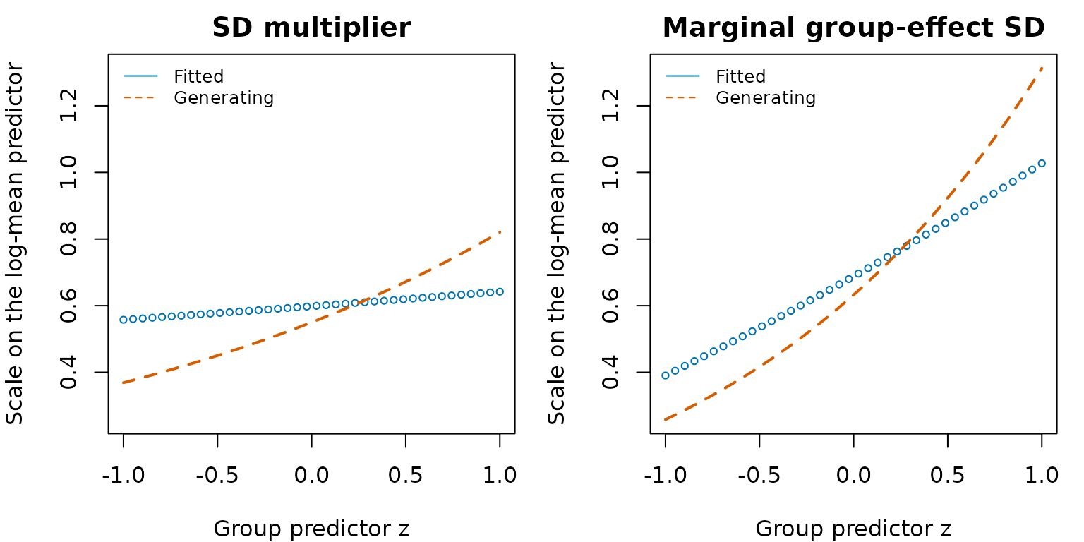
Latent group-effect scales in one synthetic Gamma data set. Circles mark model-implied values for the 40 fitted groups. Solid blue lines connect fitted values; dashed orange lines show the generating values. The left panel shows the SD multiplier, and the right includes the diagonal of K. Both are on the log-mean scale. No uncertainty bands are shown.

The points are predicted group scales, not observed response SDs or realised random intercepts. The right panel rises partly because this synthetic K has larger diagonal entries at larger z. Reading that panel alone would mix the fitted SD trend with the matrix scale.

The optional Julia interface and prediction quantities

The matched Gamma call uses the same formula, data and raw matrix. It uses maximum likelihood with a structured Laplace approximation. It needs a working Julia engine setup; this optional chunk is not run when building the article. Structured Julia fits currently require the default control, so the native se = FALSE setting is not copied across.

fit_gamma_julia <- drmTMB(
  gamma_formula, family = stats::Gamma(link = "log"), data = gamma_data,
  engine = "julia", REML = FALSE
)
coef(fit_gamma_julia, dpar = "sd_relmat(id)")
predict(fit_gamma_julia, dpar = "sd_relmat(id)")

The native and Julia Gamma fits have been checked against an independent Laplace objective on this data set. That comparison concerns this model and these point estimates. For ordinary Bernoulli and Poisson random intercepts, the Julia SD routes instead use adaptive Gauss-Hermite quadrature. A shared maximum-likelihood target does not make different integration approximations identical, so do not assume that all engine coefficients or log likelihoods will match.

In the R bridge, stored-row mean predictions on this Gamma route include the fitted group effects. Supplying newdata requests the fixed-effect prediction with random effects set to zero, including when the supplied rows happen to be the training data.

conditional_log_mean <- predict(fit_gamma_julia, dpar = "mu", type = "link")
conditional_mean <- predict(fit_gamma_julia, dpar = "mu")
fixed_effect_mean <- predict(
  fit_gamma_julia, newdata = gamma_data, dpar = "mu"
)
all.equal(conditional_mean, fitted(fit_gamma_julia))

Quantity	Interpretation
`sd_relmat(id)` response prediction	The latent SD multiplier `s_g`; multiply by `sqrt(K_gg)` for marginal group-effect SD.
Stored R bridge `mu` link prediction	The fixed linear predictor plus the fitted group contribution.
Stored R bridge `mu` response prediction	The conditional mean, obtained by applying the inverse link to that predictor.
R bridge `mu` prediction with explicit `newdata`	The fixed-effect mean with random effects set to zero.
Direct Julia `fitted()`	The direct interface’s population-level fitted value, which differs from the R bridge’s conditional output.

Setting random effects to zero does not integrate over their distribution. Under a log link, the average of exp(eta + b) generally differs from exp(eta). State which quantity a prediction plot shows.

Which source routes do these examples use?

The table below records narrowly admitted source routes for complete observed responses and fixed, finite, group-constant SD predictors. Source admission means that the interface accepts the specified model; it does not establish runtime accuracy, prediction support or calibrated uncertainty for every model with that description. The executed examples and their checks provide separate evidence.

Response	Mean effect	Native source	Julia source
Bernoulli, logit	One ordinary random intercept	Admitted within recorded scope; ML; TMB random-effect Laplace	Admitted within recorded scope; ML; adaptive Gauss-Hermite quadrature, default 5 nodes
Poisson, log	One ordinary random intercept	Admitted within recorded scope; ML; TMB random-effect Laplace	Admitted within recorded scope; ML; adaptive Gauss-Hermite quadrature, default 41 nodes
Gamma, log	One relmat random intercept; raw K	Admitted within recorded scope; ML; TMB random-effect Laplace	Admitted within recorded scope; ML; structured Laplace

Check the fit before interpreting it

The compact tables above show every check name and status without printing long diagnostic messages. The complete objects remain available as bernoulli_checks and poisson_checks; inspect, for example, bernoulli_checks[bernoulli_checks$status %in% c("warning", "error"), ] to read full details for warning and error rows. The checks cover optimizer, gradient, Hessian, standard-error, and random-effect boundary diagnostics where available. Investigate any warning or error before interpreting the coefficients. A clean diagnostic table does not establish that the SD coefficient is well identified in every design, and it does not assess repeated-sampling interval coverage.

These are likelihood-based fits. confint() returns frequentist confidence intervals; it does not return Bayesian credible intervals. This guide shows point estimates and group-level predictions only. It makes no calibrated interval claim for these examples, so do not report nominal confidence interval coverage as established by running this vignette.

Scope of these examples

The executed native examples cover Bernoulli and Poisson models with one ordinary random intercept, and a Gamma model with one related-matrix random intercept. Each models the latent SD multiplier using a group-constant predictor. The optional Julia calls concern those same selected source routes, with their own fitting approximations and output contracts. These examples do not qualify other distributions, random slopes, crossed effects, missing responses or every structured provider.

Native Bernoulli/binomial also has an explicit selector form when a scalar intercept must be named:

bf(
  y ~ x + (1 | p | group),
  sd(group, dpar = "mu", coef = "(Intercept)", block = "p") ~ w
)

That selector names one ordinary mean intercept. For other required models, check What can I fit today? and the formula grammar before fitting. This guide shows ML point estimates; it establishes neither calibrated interval coverage nor a REML result for these examples.