Fitting quantitative-genetic models • hsquared

Default path vs opt-in targets. engine = “fit” is the v0.1 univariate Gaussian REML path. Other models below use engine = “julia” with an explicit target (experimental / opt-in), except multivariate cbind(), which routes on the default call and is covered at validation scale for t = 2 unstructured. The experimental packaging label stays. See Can I fit and report this?.

This article shows the models hsquared can fit. Fitting is computed in the sibling HSquared.jl engine, so every example needs a local Julia, the JuliaCall package, and an HSquared.jl checkout (git clone https://github.com/itchyshin/HSquared.jl). After cloning, run julia --project=/path/to/HSquared.jl -e 'using Pkg; Pkg.instantiate()' once. HSquared.jl does not ship a Manifest.toml, so skipping that step fails on the first fit with a missing Optim package. The first call still precompiles (about 30 seconds after instantiate; about two minutes on a cold depot). Register the checkout with Sys.setenv(HSQUARED_JULIA_PROJECT = "/path/to/HSquared.jl") or per call via control = hs_control(engine_control = list(julia_project = "/path/to/HSquared.jl")); see the README or “Getting started” article for full setup. The code chunks are not run when this page is built (the build host has no Julia).

Gaussian fits use REML. ML is not implemented for that route: REML = FALSE is rejected, and REML = TRUE is the default. That rule applies to the default fit and to engine = "validate"; the opt-in non-Gaussian route below instead uses a Laplace marginal likelihood or a hybrid variational-plus-Laplace objective. The latter is not generally a lower bound after fixed effects are integrated.

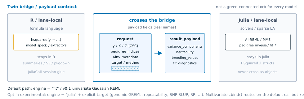
Two-column diagram of the R to Julia twin bridge. Formula language stays in R; y, X, Z CSC, pedigree indices, and target metadata cross the bridge; solvers stay in Julia; result_payload returns variance components, heritability, and breeding values. Default engine equals fit for v0.1; other targets are opt-in experimental.

What crosses the bridge vs what stays lane-local. Default engine = “fit” is the v0.1 path; opt-in targets need engine = “julia” and an explicit target. This figure does not imply production bridge coverage for every model.

Engine twin (Documenter): runnable Julia @example blocks and bridge-shaped utilities are on Quick start. Sections below map to Standard QG models, Genomic models, and Multivariate models. Live engine evidence: validation status.

The default: a univariate Gaussian animal model

This is the v0.1 model, fitted by the default hsquared() call. It estimates the additive-genetic and residual variances, heritability, and breeding values.

ped <- data.frame(
  id   = c("s1", "s2", "d1", "d2", "o1", "o2", "o3", "o4"),
  sire = c(NA, NA, NA, NA, "s1", "s1", "s2", "s2"),
  dam  = c(NA, NA, NA, NA, "d1", "d2", "d1", "d2")
)
dat <- data.frame(
  id     = ped$id,
  sex    = c("m", "m", "f", "f", "m", "f", "m", "f"),
  age    = c(4, 5, 4, 5, 1, 1, 1, 1),
  weight = c(72, 75, 65, 68, 31, 33, 35, 30)
)

library(hsquared)

fit <- hsquared(
  weight ~ sex + age + animal(1 | id, pedigree = ped),
  data = dat,
  family = gaussian(),
  REML = TRUE
)

variance_components(fit)
heritability(fit)
breeding_values(fit)   # EBVs (aliases: EBV(), BLUP())
summary(fit)

Most of the remaining models below are opt-in: they are reached through engine = "julia" with an explicit target. The one exception is the multivariate cbind() model, which routes on the default call. Being reachable by default does not drop the experimental packaging label. The Gaussian opt-in routes are REML-only; the non-Gaussian route has its own marginal-likelihood methods. Report point estimates only within a covered route; see Can I fit and report this?. The default univariate animal model and t = 2 unstructured multivariate cbind() are covered on the default call. Genomic GREML is covered at validation scale behind the explicit engine = "julia", target = "genomic" route. Four more opt-in models are covered at validation scale: each passed a pre-declared 48-seed recovery gate plus a same-estimand REML comparator: the common-environment two-effect model, arbitrary-N multi-effect, random regression k = 2, and the direct–maternal 2×2 G model. Covered at validation scale still means experimental packaging and not production. The remaining opt-in models (repeatability, the maternal two-effect leg, SNP-BLUP, single-step) stay partial.

Checking A, A-inverse, and inbreeding F

hsquared() does not return the relationship matrix A, its inverse, or inbreeding coefficients. The fit payload stores pedigree IDs; Ainv is built in Julia (ainv_status = "build_in_julia"). inbreeding() is a reserved formula term for a future effect. It is not pedigreemm::inbreeding() and it does not return F.

Compare A / A^{-1} / F against nadiv or pedigreemm through JuliaCall after the usual Julia setup (see the README). Unknown parents must be "0", not NA:

# After hs_julia_setup() or julia_setup() with HSQUARED_JULIA_PROJECT set.
JuliaCall::julia_assign("id", as.character(ped$id))
JuliaCall::julia_assign(
  "sire",
  ifelse(is.na(ped$sire), "0", as.character(ped$sire))
)
JuliaCall::julia_assign(
  "dam",
  ifelse(is.na(ped$dam), "0", as.character(ped$dam))
)
JuliaCall::julia_command(paste(
  "A = Matrix(HSquared.additive_relationship(id, sire, dam));",
  "Ainv = Matrix(HSquared.pedigree_inverse(id, sire, dam));",
  "F = collect(Float64, HSquared.inbreeding_coefficients(id, sire, dam));"
))
A <- JuliaCall::julia_eval("A")
Ainv <- JuliaCall::julia_eval("Ainv")
F <- JuliaCall::julia_eval("F")

See Function map and cheat sheet for the R-versus-Julia function table. No R accessor is added here.

Repeatability (permanent environment)

A repeated-records model with an additive-genetic effect and a permanent-environment effect that shares the animal grouping. The additive (σ²a) and permanent-environment (σ²pe) variances are only identifiable with repeated records per individual.

repeated_dat <- data.frame(
  id = rep(dat$id, each = 2),
  y = rep(dat$weight, each = 2) + c(-0.5, 0.5)
)
fit_rep <- hsquared(
  y ~ animal(1 | id, pedigree = ped) + permanent(1 | id),
  data = repeated_dat,
  control = hs_control(
    engine = "julia",
    engine_control = list(target = "repeatability")
  )
)

variance_components(fit_rep)    # animal, permanent, residual
repeatability(fit_rep)          # R = (Va + Vpe) / Vp
heritability(fit_rep)           # h2 = Va / Vp
permanent_effects(fit_rep)

Common environment

A two-effect model: an additive-genetic effect plus an independent IID environmental effect (for example a litter or cage), grouped by a separate column.

ce_dat <- data.frame(
  id = dat$id,
  y = dat$weight,
  litter = c("l1", "l1", "l2", "l2", "l1", "l2", "l1", "l2")
)
fit_ce <- hsquared(
  y ~ animal(1 | id, pedigree = ped) + common_env(1 | litter),
  data = ce_dat,
  control = hs_control(
    engine = "julia",
    engine_control = list(target = "two_effect")
  )
)

variance_components(fit_ce)     # animal, common_env, residual
common_env_effects(fit_ce)

Maternal genetic effects

The other two-effect model: a direct additive-genetic effect plus a maternal genetic effect expressed through the dam. Both carry the pedigree relationship (the maternal effect uses A₂ = pedigree A), and the dams must be animals in the animal() pedigree. This is the independent (uncorrelated) direct–maternal model; the correlated 2×2 G version is covered at validation scale (opt-in, target = "direct_maternal"; see below).

mat_dat <- data.frame(
  id = c("o1", "o2", "o3", "o4"),
  y = c(31, 33, 35, 30),
  dam = c("d1", "d2", "d1", "d2")
)
fit_mat <- hsquared(
  y ~ animal(1 | id, pedigree = ped) + maternal_genetic(1 | dam),
  data = mat_dat,
  control = hs_control(
    engine = "julia",
    engine_control = list(target = "two_effect")
  )
)

variance_components(fit_mat)    # animal, maternal_genetic, residual
maternal_effects(fit_mat)

Genomic GREML

A single genomic effect whose relationship is a user-supplied genomic relationship inverse Ginv (with id dimnames) instead of a pedigree. This estimates the genomic and residual variances, genomic heritability, and genomic breeding values (GEBVs). You can either supply a precomputed Ginv, or pass a raw marker matrix M (rows = individuals) as genomic(1 | id, markers = M) and let the engine build the genomic relationship and its inverse. Single-step can use either a supplied Hinv or the experimental constructed path single_step(1 | id, pedigree = ped, markers = M) with target = "single_step_construct". Explicit-target genomic GREML is covered at validation scale. Ordinary-call / default-route genomic activation remains held. Single-step stays exploratory.

g_dat <- data.frame(id = dat$id, y = dat$weight)
Ginv <- diag(nrow(g_dat))
dimnames(Ginv) <- list(g_dat$id, g_dat$id)
fit_g <- hsquared(
  y ~ genomic(1 | id, Ginv = Ginv),
  data = g_dat,
  control = hs_control(
    engine = "julia",
    engine_control = list(target = "genomic")
  )
)

variance_components(fit_g)      # genomic, residual
heritability(fit_g)             # genomic h2
breeding_values(fit_g)         # GEBVs

SNP-BLUP / RR-BLUP marker effects

A marker-effect model on a raw marker matrix genomic(1 | id, markers = M). You may supply the genomic and residual variances (for example from a prior GREML fit); the engine centres the markers and returns per-marker effects (marker_effects()) together with per-individual genomic breeding values. If you omit variance_components, hsquared() instead estimates the genomic and residual variances by REML from the markers (fit_snp_blup_reml). Weighted / Bayesian marker priors and comparator parity are planned.

snp_dat <- data.frame(id = dat$id, y = dat$weight)
set.seed(1)
M <- matrix(
  sample(0:2, nrow(snp_dat) * 4, replace = TRUE),
  nrow = nrow(snp_dat)
)
rownames(M) <- snp_dat$id
fit_snp <- hsquared(
  y ~ genomic(1 | id, markers = M),
  data = snp_dat,
  control = hs_control(
    engine = "julia",
    engine_control = list(
      target = "snp_blup",
      variance_components = c(sigma_g2 = 1, sigma_e2 = 2)
    )
  )
)

marker_effects(fit_snp)              # one effect per marker
marker_variance_explained(fit_snp)   # descriptive fitted-marker shares
breeding_values(fit_snp)             # per-individual GEBVs

Multivariate Gaussian animal model

The multivariate path uses a cbind() response and estimates trait-by-trait genetic and residual covariance matrices for the animal effect. It fits on the default call without an engine or target argument. The fitter is dense and validation-scale: problems above max_dense_cells (nobs^2 + nanimals^2, default 1e6; a few hundred animals at t = 2) error instead of allocating. The t = 2 unstructured route is covered on that default call (validation scale); k≥3 and diagonal genetic structure stay experimental. See Can I fit and report this?. Missing response cells are allowed; missing fixed-effect cells are rejected.

mv_dat <- dat
mv_dat$length <- c(120, 122, 118, 119, 80, 81, 83, 79)
fit_mv <- hsquared(
  cbind(weight, length) ~ sex + age + animal(1 | id, pedigree = ped),
  data = mv_dat,
  family = gaussian(),
  REML = TRUE
)

genetic_covariance(fit_mv)
genetic_correlation(fit_mv)
heritability(fit_mv)            # per-trait h2
breeding_values(fit_mv)         # animal-by-trait EBVs

The future long-format grammar animal(trait | id, pedigree = ped, cov = us()) is planned, not fitted yet. See the multivariate article for the current claim boundary.

Binary and count traits (experimental): which heritability to report

Experimental · opt-in · not coverage-calibrated. The non-Gaussian animal model fits only through engine = “julia” with target = “nongaussian”, is limited to an intercept plus one animal() term, and has not yet been checked against another program that estimates the same quantity. See Can I fit and report this? before reporting a value.

Many traits ecologists and breeders care about are not Gaussian: whether an individual survived its first winter (0/1), how many of a clutch fledged (successes out of a known number of trials), how many offspring were sired (a count). hsquared() accepts binomial(logit) and poisson(log) for these, and heritability() returns more than one number, because a heritability for a non-Gaussian trait depends on the scale you state it on.

Take fledging success in a wild bird population. Each female has a clutch of between two and seven eggs, and some number of those fledge:

bin_dat <- data.frame(
  id = ped$id,
  fledged = c(2, 3, 1, 2, 3, 2, 4, 1),
  failed = c(1, 0, 2, 1, 0, 1, 1, 2)
)
fit_fledge <- hsquared(
  cbind(fledged, failed) ~ animal(1 | id, pedigree = ped),
  data = bin_dat,
  family = binomial(),           # logit link
  control = hs_control(
    engine = "julia",
    engine_control = list(target = "nongaussian")   # marginal = "laplace" (default)
  )
)

variance_components(fit_fledge)  # V_A on the latent (logit) scale
heritability(fit_fledge)

REML = TRUE is the R front door’s current required default, so it is omitted above. It does not make this non-Gaussian fit a REML fit: this route uses a Laplace marginal likelihood (or a hybrid variational-plus-Laplace objective when selected), as stated below. The default Laplace objective integrates the intercept under a flat measure, so V_A is a REML-like Laplace estimate, not conventional Laplace-ML. At n around 800 it is expected to sit a few percent above glmer / pedigreemm / glmmTMB Laplace-ML V_A. logLik() is not comparable with glmer. The numerical method is unchanged.

heritability() returns a small table rather than a single value. For a varying-trials fit like this one it looks like:

#>            field                                     label estimate                    undefined_reason
#> 1      h2_latent            latent-scale h2 (conditional)     1.00                                <NA>
#> 2   h2_liability         liability-scale h2 (conditional)     0.20                                <NA>
#> 3 h2_observation observation-scale h2 (no scalar estimand)      NaN varying_trials_no_scalar_estimand

(The numbers are illustrative: V_A = 0.8 on the logit scale gives $0.8 / (0.8 + \pi^2/3) \approx 0.20$ ; the shape is exact.)

Which row do you report? The liability-scale one. All three rows come from the same fit on the logit scale; they differ in what goes in the denominator. Here is what each is, starting with the two that matter:

h2_liability: report this. It is the heritability of the underlying liability to fledge: the additive genetic variance on the logit scale, divided by that variance plus the logistic distribution’s own variance, $\pi^2/3 \approx 3.29$ (the distribution-specific variance of Nakagawa and Schielzeth 2010). This is the threshold-model convention the field has used since Dempster and Lerner (1950), it is the scale on which published heritabilities of survival, breeding success and disease traits are usually given, and it does not depend on how many trials each individual had. State the link when you report it: “liability-scale $h^2$ (logit link)”.
h2_observation: the NaN row. This is the heritability on the data scale, the 0/1 or proportion you actually recorded. When every individual has the same number of trials (a 0/1 survival trait, or a fixed number of attempts), this is a single number and the package reports it. When trial sizes vary, it is not a single number: a female with a clutch of two and one with a clutch of seven have different data-scale variances, so no single observation-scale $h^2$ exists for the population. hsquared therefore returns NaN with the reason varying_trials_no_scalar_estimand rather than averaging over clutch sizes and printing something that looks like an estimate. This is not a failed fit. The liability-scale row is the estimate.
h2_latent: ignore it for now. It divides the additive variance by the random latent variance only, with no $\pi^2/3$ . In the only model this path currently fits, an intercept plus one animal() term, the additive variance is the sole random component, so this row is always exactly 1. It is a bookkeeping row, not an estimate. The number to keep instead is V_A itself, from variance_components(): it is what every scale conversion, including the liability-scale row, starts from.

If you specifically need a data-scale heritability for a varying-trials trait , for example to predict a response to selection on the observed proportion, the answer is a per-individual quantity, not a population scalar. Compute it from the latent-scale V_A and intercept with the conversions in de Villemereuil et al. (2016) (the QGglmm package), which integrate over the link for a stated trial count, or refit on a subset with a common trial count.

Two more things to know about this path. The engine can approximate the likelihood in two ways: marginal = "laplace" (the default) or marginal = "variational" (aliases "la"/"va", which uses a Gaussian variational approximation for genetic effects and a Laplace correction for fixed effects). The latter is not guaranteed to be a lower bound on the integrated likelihood. Their logLik() and AIC() values are not comparable with each other, nor with the REML values from the Gaussian fits above, nor with glmer Laplace-ML. And Poisson fits report h2_latent and a count-scale h2_observation only; there is no liability scale for a count.

References. Dempster, E. R. & Lerner, I. M. (1950) Heritability of threshold characters. Genetics 35, 212–236. Nakagawa, S. & Schielzeth, H. (2010) Repeatability for Gaussian and non-Gaussian data: a practical guide for biologists. Biological Reviews 85, 935–956. de Villemereuil, P., Schielzeth, H., Nakagawa, S. & Morrissey, M. (2016) General methods for evolutionary quantitative genetic inference from generalized mixed models. Genetics 204, 1281–1294.

What is fitted, and what is planned

Before extracting an estimate, read fit diagnostics and plots. Before reporting one, return to Can I fit and report this?.

formula_status() and validation_status() report, from R, exactly which terms fit and how each capability is validated.

library(hsquared)

## hsquared is an experimental 0.9.0 release (not production; CRAN availability is tracked separately). Default fitting needs Julia + HSquared.jl; preview with hs_control(engine = "validate").
## What you may report is listed on Can I fit and report this? -- not in validation_status(). Intervals are not coverage-calibrated.
## See https://itchyshin.github.io/hsquared/articles/current-limits.html

formula_status()

## <hs_formula_status>
##   default: animal(); cbind()
##   opt-in: 
##     permanent(); common_env(); maternal_genetic(); (1 | group);
##     animal(rr()); metafounder(); relmat(); precision(); genomic();
##     single_step()
##   reserved/planned: 14 reserved, 5 planned (error before fitting)
##   fences: $current_behavior
##                                                                            term
##                                                  animal(1 | id, pedigree = ped)
##                         animal(1 | id) with data = hs_data(..., pedigree = ped)
##                                                               permanent(1 | id)
##                                                           common_env(1 | group)
##                                                       maternal_genetic(1 | dam)
##                                                                     (1 | group)
##                           animal(rr(covariate, order = 2) | id, pedigree = ped)
##                                                           maternal_env(1 | dam)
##                                      paternal_genetic(1 | sire, pedigree = ped)
##                                                          paternal_env(1 | sire)
##                                                        group(1 | genetic_group)
##                                                   unknown_parent_group(1 | upg)
##               metafounder(1 | id, pedigree = ped, group = group, Gamma = Gamma)
##                                                              inbreeding(1 | id)
##                                                  cytoplasmic(1 | maternal_line)
##                         imprinting(1 | id, pedigree = ped, parent = "maternal")
##                                               dominance(1 | id, pedigree = ped)
##                                               epistasis(1 | id, pedigree = ped)
##                                                           relmat(1 | id, K = K)
##                                                        precision(1 | id, Q = Q)
##                                                    genomic(1 | id, Ginv = Ginv)
##                                                    genomic(1 | id, markers = M)
##                                                single_step(1 | id, Hinv = Hinv)
##                                single_step(1 | id, pedigree = ped, markers = M)
##     single_step(1 | id) with data = hs_data(..., pedigree = ped, genotypes = M)
##  single_step(1 | id, pedigree = ped, markers = M, group = group, Gamma = Gamma)
##                                                    markers(M, model = "random")
##                                                marker_scan(M, map = marker_map)
##                                      qtl_scan(position, genotype_probs = probs)
##                          cbind(trait1, trait2) ~ animal(1 | id, pedigree = ped)
##                                  animal(trait | id, pedigree = ped, cov = us())
##                                animal(trait | id, pedigree = ped, cov = diag())
##                        animal(trait | id, pedigree = ped, cov = lowrank(K = 2))
##                             animal(trait | id, pedigree = ped, cov = fa(K = 2))
##                                    missing = miss_control(response = "include")
##                          mi(x) with missing = miss_control(predictor = "model")
##  syntax_status                                      fitting_status
##         parsed                               fitted (v0.1 default)
##         parsed                               fitted (v0.1 default)
##         parsed                       fitted (opt-in repeatability)
##         parsed                  fitted (opt-in common-environment)
##         parsed                            fitted (opt-in maternal)
##         parsed                        fitted (opt-in multi-effect)
##         parsed                   fitted (opt-in random-regression)
##       reserved                                       not available
##       reserved                                       not available
##       reserved                                       not available
##       reserved                                       not available
##       reserved                                       not available
##         parsed          fitted (opt-in supplied-Gamma metafounder)
##       reserved                                       not available
##       reserved                                       not available
##       reserved                                       not available
##       reserved                                       not available
##       reserved                                       not available
##         parsed fitted (opt-in supplied relationship, experimental)
##         parsed    fitted (opt-in supplied precision, experimental)
##         parsed   fitted (opt-in genomic, covered validation-scale)
##         parsed                  fitted (opt-in genomic / SNP-BLUP)
##         parsed                         fitted (opt-in single-step)
##         parsed            fitted (opt-in single-step construction)
##         parsed     fitted (opt-in single-step bundle construction)
##         parsed              fitted (opt-in supplied-Gamma H^Gamma)
##       reserved                                       not available
##       reserved                                       not available
##       reserved                                       not available
##         parsed        fitted (default route, covered multivariate)
##        planned                                       not available
##        planned                                       not available
##        planned                                       not available
##       reserved                                       not available
##        planned                                       not available
##        planned                                       not available

validation_status()

## <hs_validation_status>
##   validation: status table only; checks are run by tests and CI
##   public claims: developer evidence table, not the user-facing list
##   of what you may report; see Can I fit and report this?
##   this table is not the full list of covered routes -- opt-in
##   random_regression (k = 2) and direct_maternal are covered with no
##   row yet; see the current-limits article
##   shown below: `capability_label` (current wording); look rows up by
##   the stable `capability` id that dated evidence records cite
##                                                                                                                              capability_label
##                                                                                                               tiny deterministic Ainv fixture
##                                                                                                               Mrode9 pedigree Ainv comparator
##                                                                                                       supplied-variance Henderson MME fixture
##                                                                                                               sparse REML likelihood identity
##                                                                                                         Mrode-style supplied-variance outputs
##                                                                                                   experimental sparse REML estimator (opt-in)
##                                                                                                 experimental repeatability estimator (opt-in)
##  two-effect / arbitrary-N independent-effect estimator (opt-in; covered: common-env + (1|g) iid / A2=I; experimental: maternal / A2=pedigree)
##                                                                   experimental supplied-relationship estimator (opt-in: genomic, single-step)
##                                                       experimental SNP-BLUP marker-effect model (opt-in; supplied-variance or REML-estimated)
##                                                                                      experimental multivariate REML estimator (default route)
##                                                                                  univariate Gaussian animal-model fit (default path, AI-REML)
##                                                                                       external published-REML recovery (gryphon, R reference)
##                                                                                     known-truth DGP variance-component recovery (R reference)
##                                                                                                             Mrode fitted animal-model outputs
##                                                                                                                      ASReml comparison policy
##                                                                                                          BLUPF90/DMU/WOMBAT comparison policy
##                                                                                                                         XSim simulation truth
##                                                                                                               genomic and QTL/eQTL validation
##                                                                                                           GLLVM-style multivariate validation
##                                                                                                                    CPU/GPU backend comparison
##     phase  status
##   Phase 1 partial
##   Phase 1 partial
##   Phase 1 partial
##   Phase 1 partial
##   Phase 1 partial
##   Phase 1 partial
##   Phase 2 partial
##   Phase 2 covered
##   Phase 5 covered
##   Phase 5 partial
##   Phase 3 covered
##   Phase 1 covered
##   Phase 1 covered
##   Phase 1 covered
##   Phase 1 planned
##   Phase 1 planned
##   Phase 1 planned
##  Phase 5+ planned
##  Phase 5+ planned
##   Phase 6 planned
##  Phase 7+ planned

What you may report is listed on Can I fit and report this?, not in validation_status(). That function is a developer evidence table; an absent row is not an absent covered route. The four opt-in models listed as covered above (two_effect common-env leg, multi_effect, random_regression, direct_maternal) are covered at validation scale, as is explicit-target genomic GREML. The t = 2 unstructured multivariate cbind() model is covered on the default call. The remaining opt-in models (repeatability, the maternal two-effect leg, SNP-BLUP, single-step) remain partial until their HSquared.jl gates and external comparators are signed off. Structured multivariate formula grammar and broad factor-analytic covariance remain on the roadmap. A bounded four-trait Gaussian FA fit and a bounded Poisson genetic GLLVM fit are available through explicit expert controls; see Multivariate Gaussian animal models and Genetic GLLVM opt-in. Further non-Gaussian families (negative binomial, ordinal, zero-inflated, hurdle), unusual-inheritance, and GPU models remain on the roadmap.