Getting started with hsquared

Experimental 0.9.0 release — not production. CRAN submission, acceptance, and public availability are separate states. Version tracks covered capability (a validation status: the named model type, or route, has a recovery gate and an external comparator), not surface area. public_covered_count is 7 (multivariate + explicit 0.7 genomic GREML) — a claims-register ledger total, not a function you can call. Fitting needs a local Julia and an HSquared.jl checkout; it is not registered in Julia General. Do not use install-by-name (Pkg.add("HSquared")). Read Can I fit and report this? before putting a number in a paper.

Default univariate path shown. Genomic and QTL routes are not this arrow. Multivariate cbind() is a separate path — read Can I fit and report this? before reporting it.

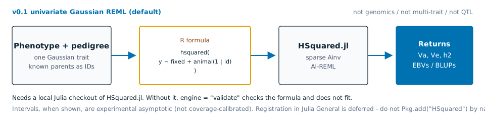
hsquared is the R interface for a Julia-backed animal model. The first working path is one Gaussian trait, one animal() term, REML. This page uses a four-animal pedigree so the first block runs without Julia. n = 4 is a syntax demo, not a number for a paper.

library(hsquared)
#> hsquared is an experimental 0.9.0 release (not production; CRAN availability is tracked separately). Default fitting needs Julia + HSquared.jl; preview with hs_control(engine = "validate").
#> What you may report is listed on Can I fit and report this? -- not in validation_status(). Intervals are not coverage-calibrated.
#> See https://itchyshin.github.io/hsquared/articles/current-limits.html

ped <- data.frame(
  id   = c("sire", "dam", "off1", "off2"),
  sire = c(NA, NA, "sire", "sire"),
  dam  = c(NA, NA, "dam", "dam")
)
dat <- data.frame(
  id     = c("sire", "dam", "off1", "off2"),
  sex    = c("m", "f", "m", "f"),
  weight = c(42, 38, 40, 37)
)

Check the model (no Julia)

hsquared(
  weight ~ sex + animal(1 | id, pedigree = ped),
  data = dat,
  control = hs_control(engine = "validate")
)
#> Validated the v0.1 animal-model contract; no model was fitted (`engine = "validate"`). Julia fit target: `HSquared.fit_animal_model(y, X, Z, Ainv; method = :REML)`. The validated spec is returned invisibly as a named list; assign it to inspect the parsed contract (e.g. `spec$bridge$target`).

model_spec(
  weight ~ sex + animal(1 | id, pedigree = ped),
  data = dat
)
#> <hs_model_spec>
#>   response: weight
#>   family: gaussian(identity)
#>   method: REML
#>   observations: 4; fixed columns: 2; animal IDs: 4
#>   animal term: animal(1 | id, pedigree = ped); group: id
#>   random design: sparse Z with 4 nonzero entries
#>   Ainv: build_in_julia
#>   fitting: not run by `model_spec()`

hsquared(..., control = hs_control(engine = "validate")) confirms the formula and data. model_spec() shows the parsed design and the engine target that would be called. Nothing is fitted.

Fit (needs the Julia engine)

Installing hsquared (remotes::install_github("itchyshin/hsquared"); pak::pak("itchyshin/hsquared") is equivalent) gives you the R interface only. Those commands do not build vignettes, so vignette("hsquared") is empty after install; this page also lives on the website. Fitting needs a local Julia 1.10 or later with julia on PATH, the JuliaCall R package, and an HSquared.jl checkout (git clone https://github.com/itchyshin/HSquared.jl). After cloning, install the recorded Julia dependencies once:

julia --project=/path/to/HSquared.jl -e 'using Pkg; Pkg.instantiate()'

HSquared.jl does not ship a Manifest.toml, so skipping Pkg.instantiate() fails on the first fit with a missing Optim package. The first call still precompiles (about 30 seconds after instantiate; about two minutes on a cold depot). Register the checkout with Sys.setenv(HSQUARED_JULIA_PROJECT = "/path/to/HSquared.jl"), or per call:

fit <- hsquared(
  weight ~ sex + animal(1 | id, pedigree = ped),
  data = dat,
  control = hs_control(
    engine_control = list(julia_project = "/path/to/HSquared.jl")
  )
)

Once the engine is registered, the same call as the validate block attempts a fit. The first fit in a session takes about 30 s while Julia starts and compiles. Later fits take under a second for a few hundred animals. The call prints no progress, so the first one can look frozen. n = 4 may not converge. If fit_diagnostics() says converged is FALSE, do not read heritability() as a result – a near-zero value is not h^2 = 0. heritability() warns when the fit failed. The successful first path on this page is the validate block above.

fit <- hsquared(
  weight ~ sex + animal(1 | id, pedigree = ped),
  data = dat
)

fit_diagnostics(fit)
heritability(fit)          # warns if the fit did not converge
variance_components(fit)
breeding_values(fit)

Without the engine, that default call errors with install guidance rather than silently degrading. Until then, engine = "validate" is the successful path.

ML is not implemented. REML = FALSE is rejected; use REML = TRUE (the default). That is the same rule for the default fit and for engine = "validate".

After this works

Read Can I fit and report this? before putting a number in a paper. Point estimates are reportable only on covered routes; intervals are experimental and not coverage-calibrated. Named univariate pedigree intervals are only classified as directional-conservative: they tend to be at least as wide as a nominal 95% interval on the measured designs, not “never under-cover”.

The gryphon worked example is a later teaching dataset (supplied relationship, compare to sommer), not this first example.

formula_status() lists which terms parse and which fit. permanent(), common_env(), and maternal_genetic() are parsed; they fit only with a named target =. The default hsquared() call names that target and stops. See Fitting models. Continue in the same order: Choose a model, Fit, Diagnose, then Report. Read Progression & evidence when you need the history behind a route label rather than a current reporting decision.

Twin-package flow

R formula + data
-> R validation and model specification
-> R bridge payload: y, X, sparse Z, method, IDs, pedigree metadata
-> HSquared.jl sparse engine
-> compact result
-> hsquared_fit object
-> R summaries, extractors, plots, and diagnostics

R owns the friendly interface. Julia owns the fit.

Engine-side walkthrough (pedigree utilities, bridge-shaped specs, experimental fitters): HSquared.jl Quick start. Status before reporting: engine validation status.