Visualizing an animal model

Intervals: asymptotic / experimental · not coverage-calibrated. Figures below are from small illustrative fit objects (no engine at build time). Subtitles and captions must be read as product chrome, not as a live analysis.

Use this page after fitting and before extracting a result for a paper. The current-limits page decides what may be reported; a plot or a converged optimizer does not broaden that permission.

hsquared ships a small ggplot2 visualization layer in the style of the brms/bayesplot ecosystem (and consistent with the sister packages drmTMB and gllvmTMB). Every figure is produced by an autoplot() method, returns a ggplot object you can theme and extend, and is uncertainty-first: where the fit carries the experimental standard errors, reliabilities, or prediction error variances, the figure shows them — clearly labelled experimental and asymptotic.

In your own analysis, fit is the object returned by hsquared():

fit <- hsquared(
  weight ~ sex + animal(1 | id, pedigree = ped),
  data = dat, family = gaussian(), REML = TRUE
)
autoplot(fit, "variance")

Check the fit before plotting

Start with the exported diagnostic table. It reports the current fit payload; it does not refit, validate a route, or turn a converged optimizer into broader reporting permission. Read any convergence or boundary indication before extracting a number, then return to current limits for the route-specific reporting scope.

fit_diagnostics(fit)

The figures below are rendered from small illustrative fit objects so the article is self-contained (no engine required to build the page); the autoplot() calls are exactly what you would run on a real fit.

Variance components and heritability

autoplot(fit, "variance") draws a horizontal forest of the variance components and per-trait h², with experimental asymptotic intervals (± 1.96 · SE) when the fit carries standard errors. These are not coverage-calibrated 95% CIs.

autoplot(fit, "variance")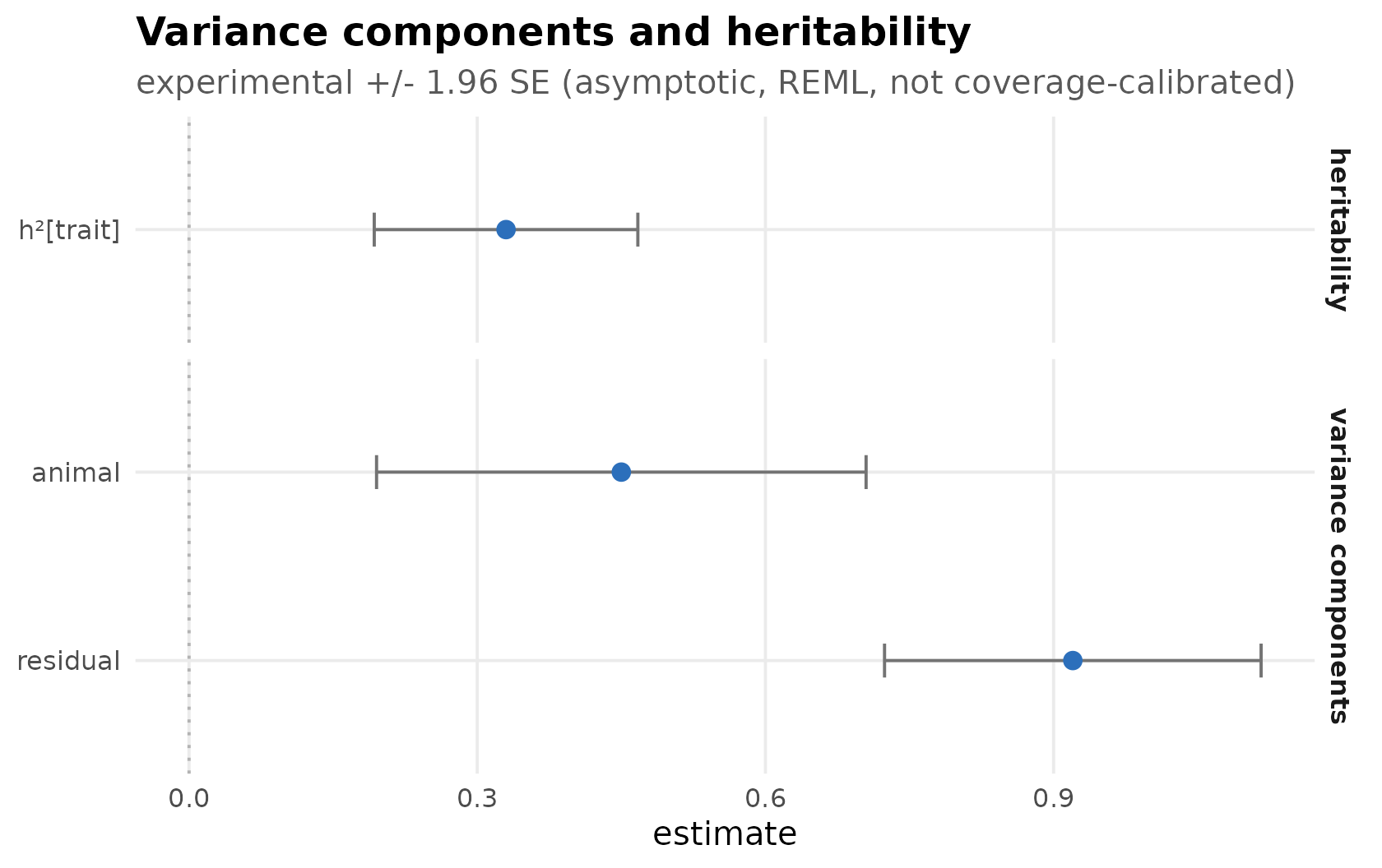

Illustrative data. Horizontal forest of animal and residual variance and heritability with experimental asymptotic error bars, labelled not coverage-calibrated.

Breeding values

autoplot(fit, "breeding_values") draws the sorted estimated breeding values as a caterpillar, with ± 1.96 · √PEV bands when prediction error variances are available (faceted by trait for multivariate fits). Caption: MME/PEV at fitted variances — not a sampling distribution of h².

autoplot(fit, "breeding_values")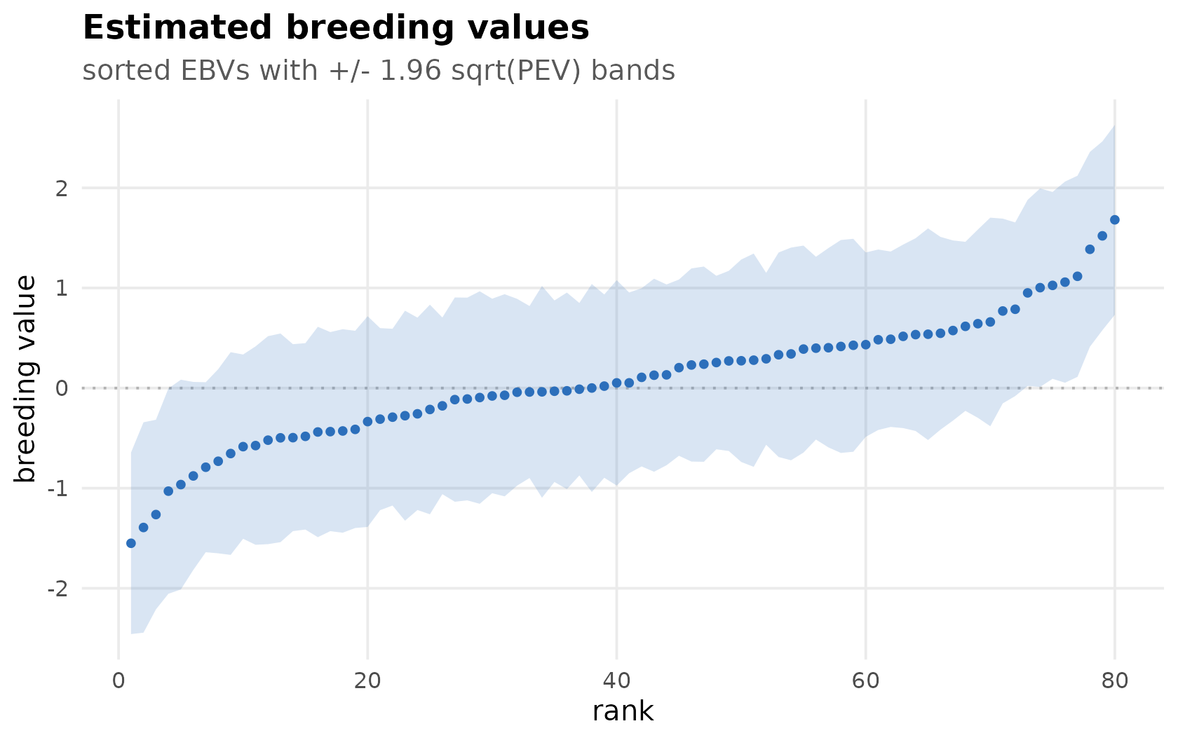

Illustrative data. Sorted EBVs with PEV bands — prediction-error grain, not a heritability CI.

Genetic correlation (G)

autoplot(fit, "g_matrix") draws the genetic-correlation matrix of an opt-in multivariate fit. It is rotation-invariant — correlations do not depend on the factor rotation — so it is well defined for any multivariate fit; raw factor loadings are never plotted (the ratified cross-lane convention).

autoplot(fit_mv, "g_matrix")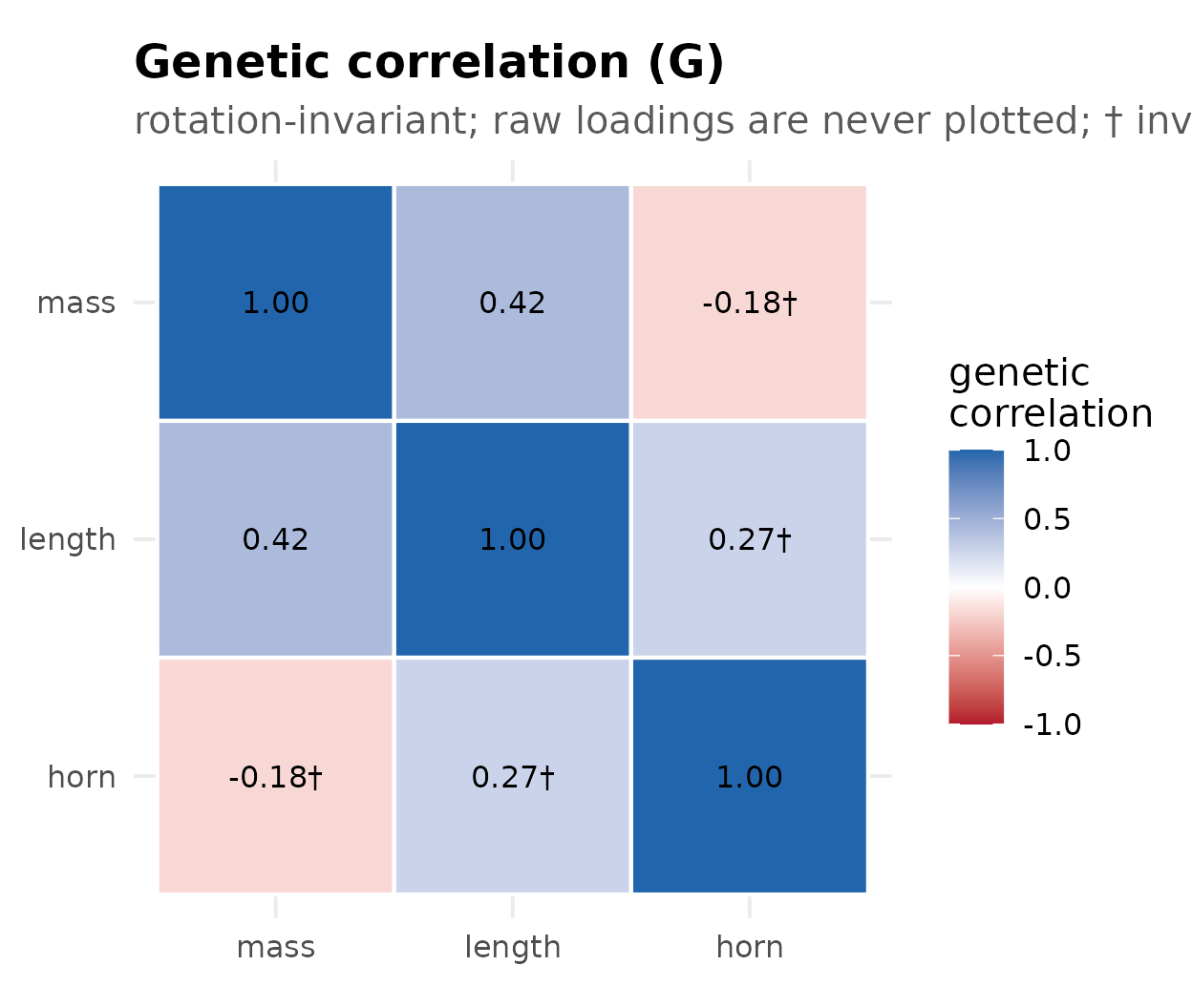

Illustrative data. Experimental / opt-in multivariate genetic-correlation triangle; rotation-invariant, loadings not shown; low-h² cells flagged imprecise.

The heatmap also flags off-diagonal cells that involve a low-h² trait (where the genetic correlation is imprecise); pass low_h2 = to set the threshold.

Genetic eigenstructure (G geometry)

autoplot(fit_mv, "g_geometry") draws a scree of the rotation-invariant genetic eigenstructure — the eigenvalues of G (variance per genetic axis) with the percent variance explained. Axis directions and loadings are never drawn: they are rotation-arbitrary and span-ambiguous under repeated eigenvalues.

autoplot(fit_mv, "g_geometry")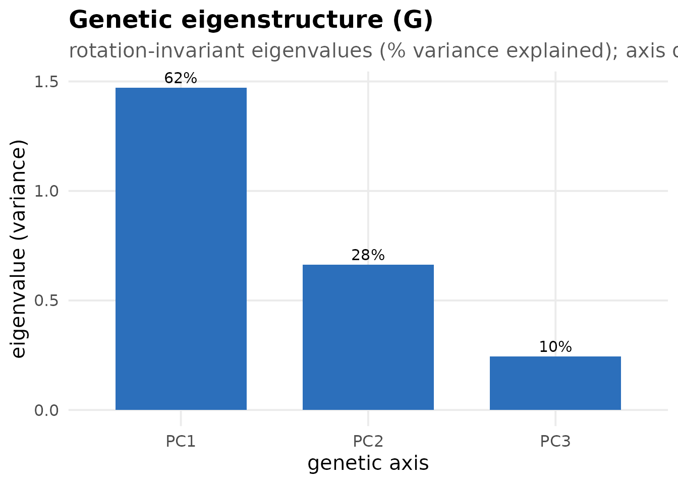

Marker scan (Manhattan)

autoplot() on the result of gwas(fit, markers) draws a Manhattan plot. The p-values are nominal Wald p-values and are not genome-wide calibrated — the figure carries that banner, and the dashed line is a plain Bonferroni reference, not a validated genome-wide threshold. HSquared.jl PR #134 adds a fixed-panel calibration smoke harness on the engine side, but this plot still does not carry an activated R significance threshold.

autoplot(gw)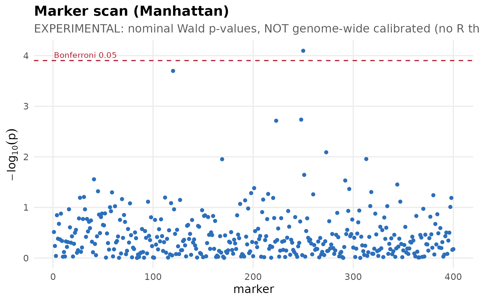

Illustrative data. Manhattan of nominal Wald p-values; dashed Bonferroni is a reference, not a validated genome-wide threshold.

Marker scan (QQ)

autoplot(gw, "qq") draws the QQ plot of the scan: observed versus expected −log10(p) with a y = x null reference and the genomic-inflation lambda_GC as a diagnostic annotation. As with the Manhattan, the p-values are nominal Wald p-values and are not genome-wide calibrated.

autoplot(gw, "qq")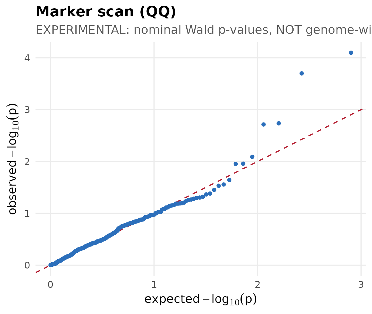

Illustrative data. QQ plot of nominal Wald p-values; not genome-wide calibrated.

Reaction norms (random regression)

For a random-regression fit, autoplot(fit, "reaction_norm") draws the genetic-variance and heritability trajectories across the covariate. The h²(t) trajectory is experimental: with a homogeneous residual and no permanent-environment term it can overstate heritability for repeated-records designs.

autoplot(fit_rr, "reaction_norm")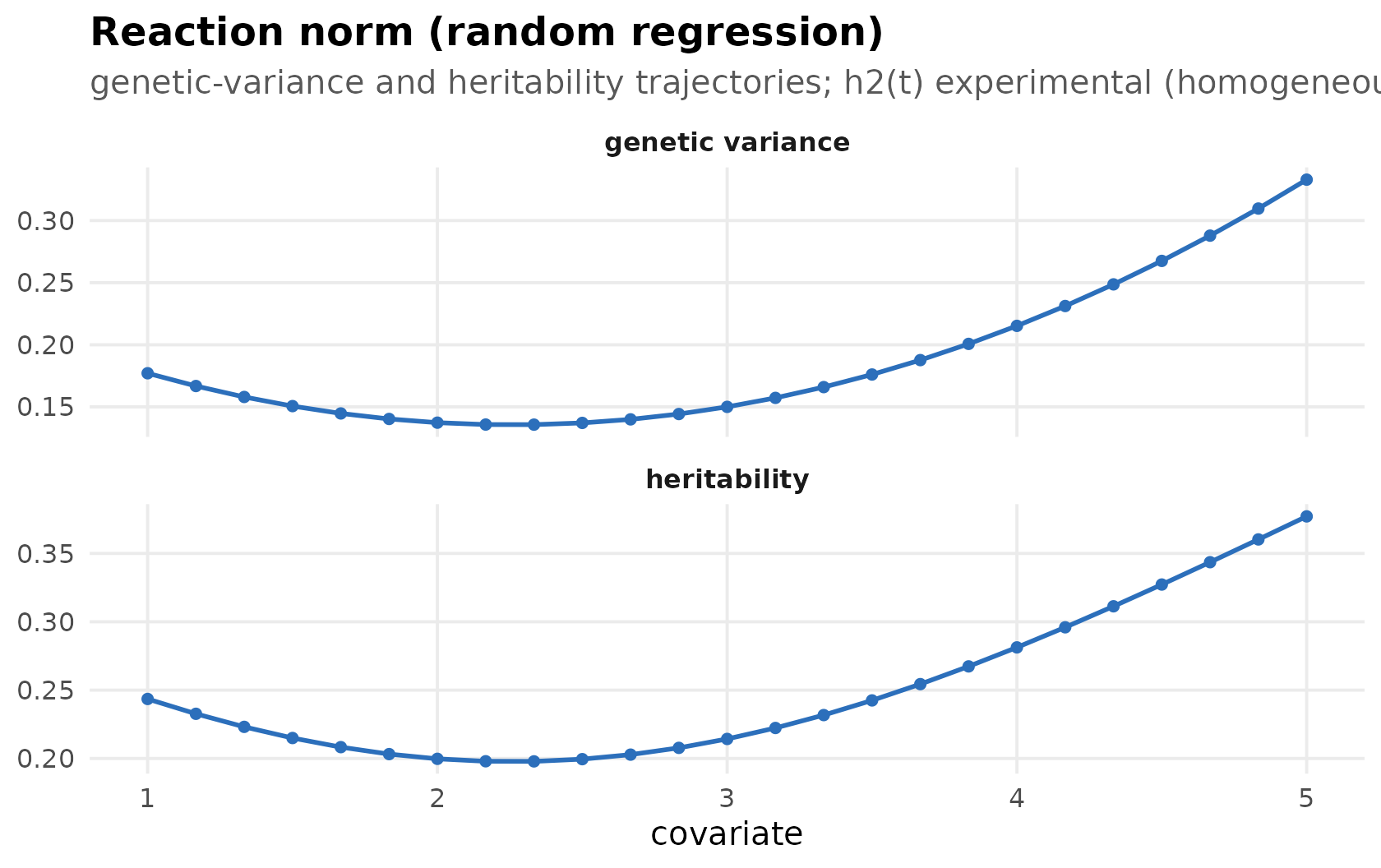

autoplot(fit, "rr_eigenfunctions") draws the rotation-invariant eigenfunctions ψ_j(t) of the coefficient covariance K_g as covariate functions, faceted by axis and labelled with the percent genetic variance. Eigenfunction signs are arbitrary and the curves are span-ambiguous under repeated eigenvalues, so do not over-read their direction.

autoplot(fit_rr, "rr_eigenfunctions")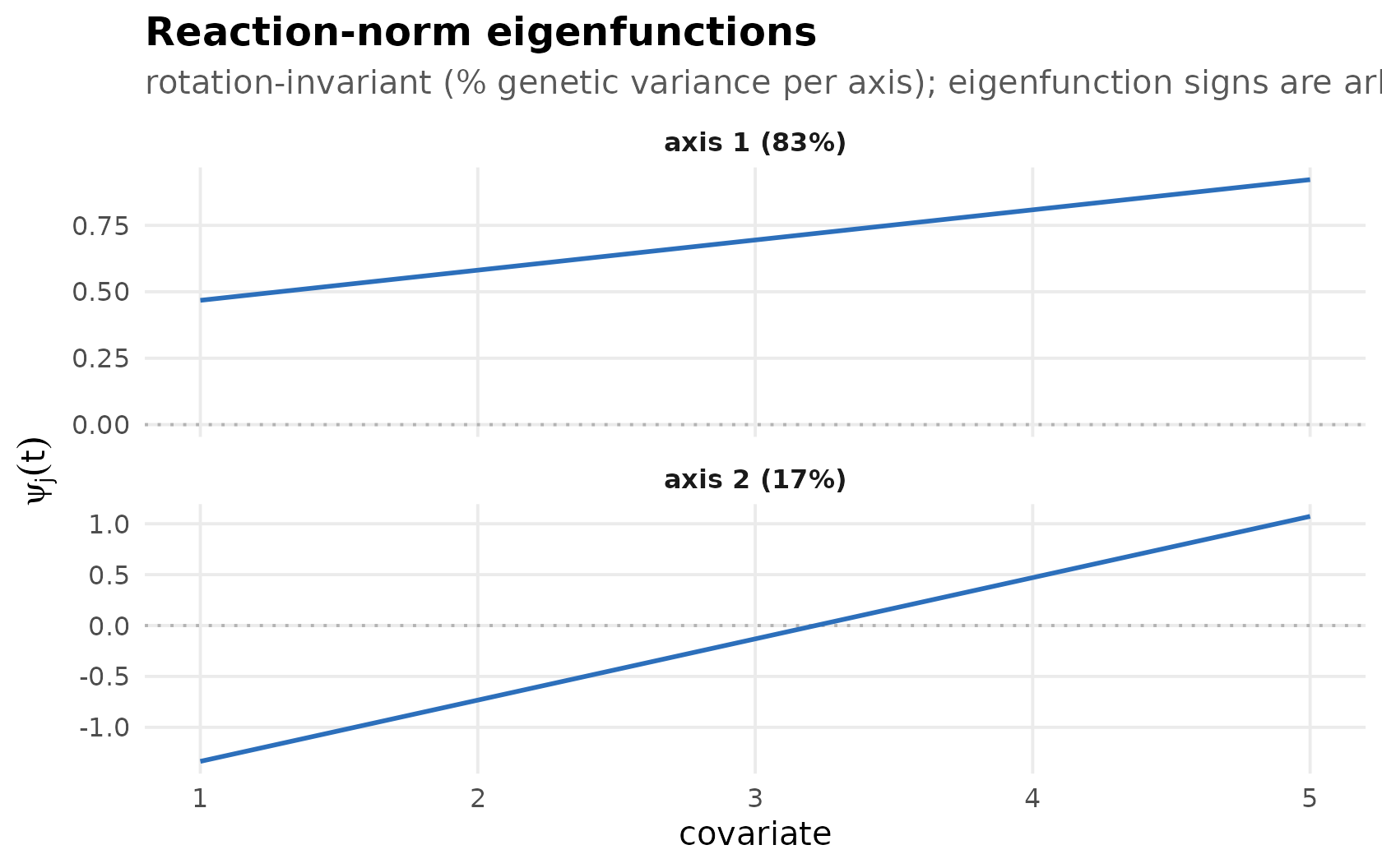

autoplot(fit, "rr_surface") draws the genetic covariance surface S(s, t) = φ(s)′ K_g φ(t) over the covariate grid as a heatmap; pass correlation = TRUE for the genetic-correlation surface.

autoplot(fit_rr, "rr_surface")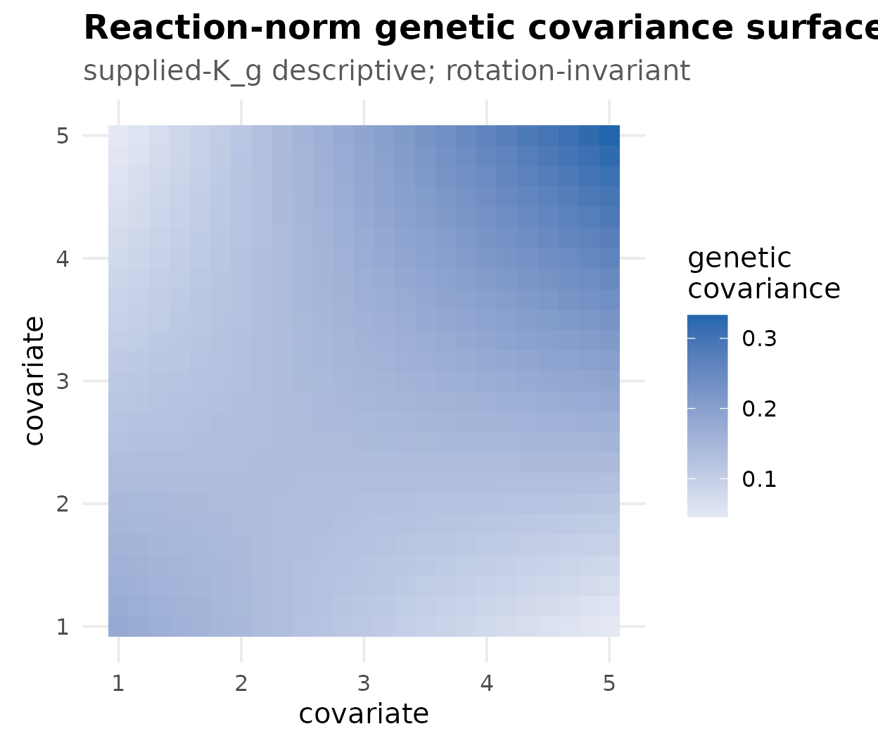

Known-truth recovery studies

hs_recovery_forest() visualizes a known-truth recovery study (such as data-raw/multivariate-recovery-study.R): each target’s bias with its ± 2 · MCSE interval. Intervals that cover zero indicate no detectable bias.

recovery <- data.frame(
  target = c("G0[1,1]", "G0[2,1]", "G0[2,2]", "R0[1,1]", "R0[2,1]",
             "R0[2,2]", "rg", "h2[1]", "h2[2]"),
  bias = c(-0.00395, 0.00621, -0.01459, 0.01171, -0.01223, -0.00106,
           0.01652, -0.00756, -0.00676),
  mcse = c(0.02221, 0.01397, 0.01726, 0.01387, 0.01164, 0.01199,
           0.01553, 0.00817, 0.00697)
)
hs_recovery_forest(recovery)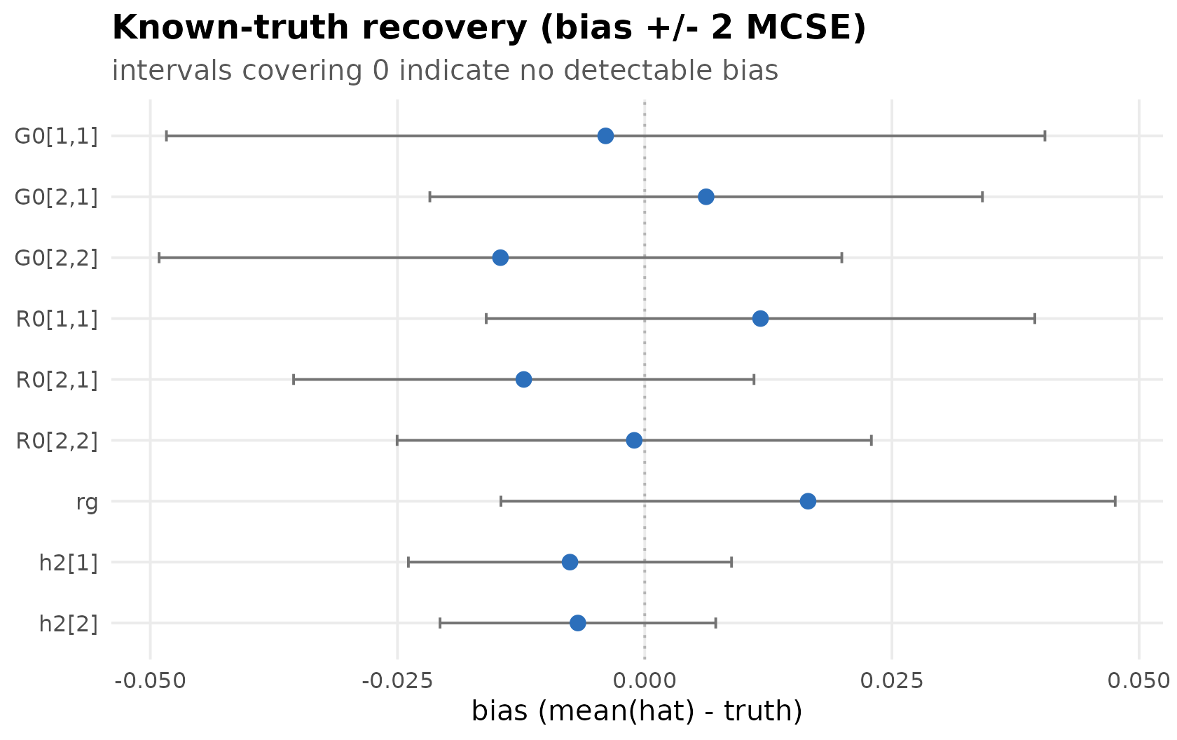

Theming

Every figure returns a ggplot object, so you can restyle it with the usual ggplot2 grammar, and theme_hsquared() is exported for reuse:

autoplot(fit, "variance") +
  ggplot2::labs(title = "My trait") +
  theme_hsquared(base_size = 14)